Lecture 10
Strings and pattern matching
Strings
-
Sequence of characters
-
Alhpabet - set of possible characters for a family of strings
- {0,1} (binary alphabet)
- {A, C, G, T} (DNA structures)
-
Substring
S[i,...j] -
Prefix: substring of the type
S[0..i] -
Suffix: substring of the type
S[i...m-1]
Pattern Matching Problem
- Given string
T(text) and P(pattern)- Find substring of
Tequal toP
- Find substring of
Brute force pattern matching
- Compare the pattern P with the text T for each possible shift of P relative to T
Algorithm BruteForceMatch(T, P)
    Input: text T of size n and pattern P of size m
    Output: starting index of a substring of T equal to P
        or -1 if no such substring exists

    for  i <- 0 to n – m  do
    { test shift i of the pattern }
        j <- 0
        while  j < m OR T[i + j] = P[j]  do
            j <- j + 1
        if  j = m  then
            return  i {match at i}
        else
            break while loop {mismatch}
        return  -1 {no match anywhere}
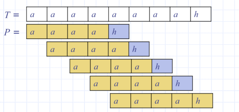
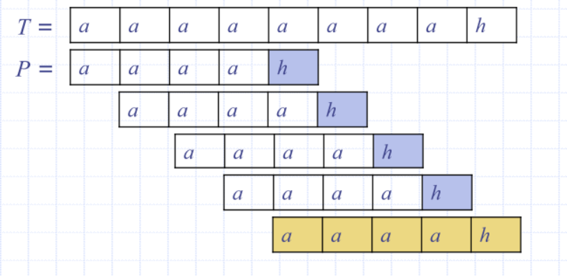
- Brute-force pattern matching runs in time O(nm)
- Example of worst case:
- T = aaa … ah and P = aaah
Can we do better?
- Boyer-Moore pattern matching algorithm
- Attempts to improve the Brute-Force
approach by using two heuristics
- Looking-glass heuristic
- Character-jump heuristic
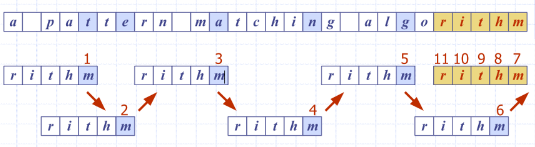
Boyer-Moore: Looking-Glass Heuristic
- Compare P with a subsequence of T moving backwards
Boyer-Moore: Character-Jump Heuristic
-
When a mismatch occurs at T[i] = c
- if P contains c, shift P to align the last occurrence of c in
P with T[i]

- if P contains c, shift P to align the last occurrence of c in
P with T[i]
-
Else, shift P to align P[0] with T[i + 1]
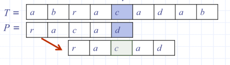
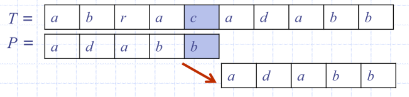
Example
- at the end, mismatches on a h and realigns
Terminology (used further)
| symbol | def'n |
|---|---|
| alphabet | |
| Pattern | |
| full string (to pattern match) | |
| $ | |
| $ |
Last-Occurrence Function
-
Boyer-Moore’s algorithm preprocesses the pattern P and the alphabet to build the last-occurrence function L mapping to integers, where is defined as
- largest index i such that P[i] = c or
- -1 if no such index exists
-
Example
Then:
| a | b | c | d | |
|---|---|---|---|---|
| 4 | 5 | 3 | -1 |
Last Occurrence Function
Can be represented by an array indexed by the numeric codes of the characters
- computed in time, where
mis the size ofPandsis the size of - accessed in O(1) time
Algorithm BoyerMooreMatch(T, P, S)
L <- lastOccurenceFunction(P, S)
i <- m - 1   { m is size of P }
j <- m - 1

repeat
    if T[i] = P[j] then
        if  j = 0 then
            return  i { match at i }
        else
            i <- i - 1
            j <- j - 1
    else
        { character-jump }
        l <- L[T[i]]
        i <- i + m – min(j, 1 + l)
        j <- m - 1
    until  i > n - 1
    return -1 { no match}
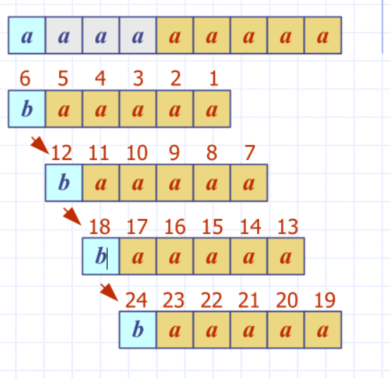
Performance analysis
- Runs in time
- Could potentially be worst than brute force time
- Example of worst case
- T = aaa … a
- P = baaa
- Boyer-Moore’s algorithm is significantly faster than the brute-force algorithm
Worst case example
Knuth-Morris-Pratt (KMP) Algorithm
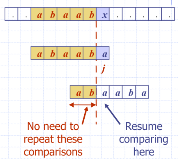
- Compares the pattern to the text left-to-right
- but shifts the pattern more intelligently than the brute-force algorithm
- When a mismatch occurs, what is the most we can shift the pattern so as to avoid redundant comparisons?
- Answer: the largest prefix of
P[0...j-1]that is a suffix ofP[1...j-1]- repeat redundant patterns
- computes a failure function
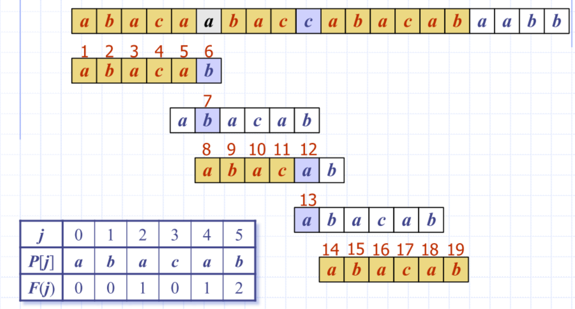
KMP failure function
- KMP algorithm preprocesses the pattern
- Failure function F(j) is defined as the size of the largest prefix of P[0..j] that is also a suffix of P[1..j]
- KMP algorithm modifies the brute-force algorithm so that if a mismatch occurs at P[j] T[i] we set j <- F(j - 1)
J |
0 | 1 | 2 | 3 | 4 | 5 |
|---|---|---|---|---|---|---|
P[j] |
a | b | a | a | b | a |
F(j) |
0 | 0 | 1 | 1 | 2 | 3 |
KMP Algorithm
- Failure function can be represented by an array and can be computed in time
- Each iteration of the while-loop, either
- i increases by one, or
- shift amount i - j increases by at least one (observe that F(j - 1) < j)
- Hence, there are no more than 2n iterations of the while-loop
- Thus, KMP’s algorithm runs in optimal time
Algorithm KMPMatch(T, P)
F <- failureFunction(P)
i <- 0
j <- 0
while  i < length(T)
    if  T[i] = P[j]  then
        if  j = length(P) - 1  then
            return  i - j { match }
        else
            i <- i + 1
            j <- j + 1
else
    if  j > 0 then
        j <- F[j - 1]
    else
        i <- i + 1
return  -1 { no match }
Example
Tries - Retrieval Tries
Preprocessing steps
- Preprocessing the pattern speeds up pattern matching queries
- After preprocessing the pattern, KMP’s algorithm performs pattern matching in time proportional to the text size
- If text is large, and searched often, preprocess the text (create and index)
- trie supports pattern matching queries in time proportional to the pattern size
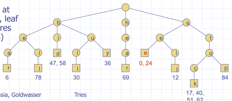
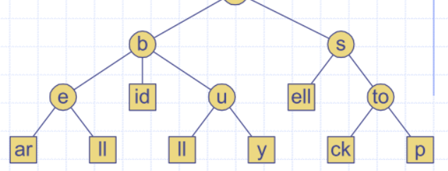
Standard trie for the set of strings S = { bear, bell, bid, bull, buy, sell, stock, stop }
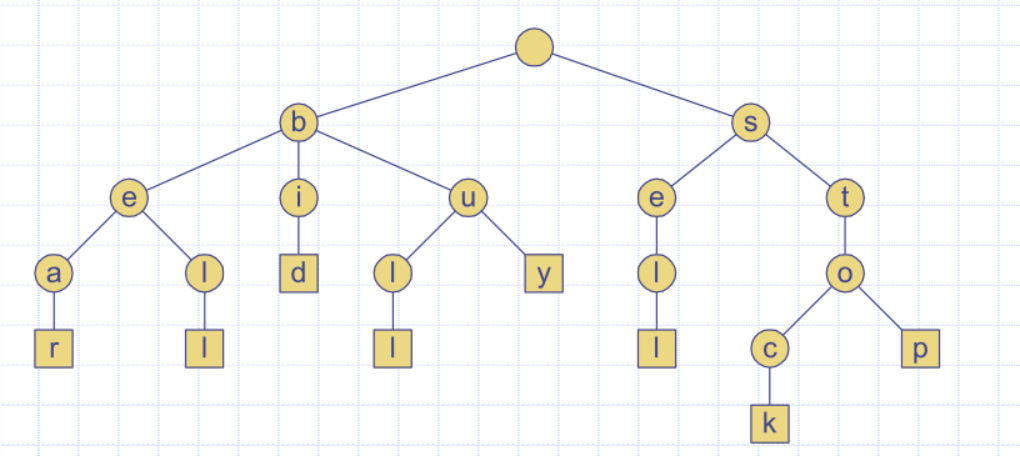
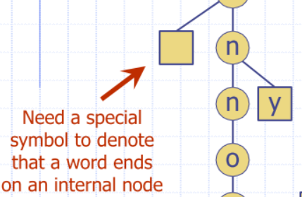
- sometimes represented as a special symbol to denote that a word ends on an internal node
Analysis of standard tries
ntotal size of the strings in Smsize of the string parameter of the (e.g. search) operationdsize of the alphabet (mostly fixed? i.e. acgt)- uses
O(n)space - supports searches, insertions and deletions in time
O(dm)
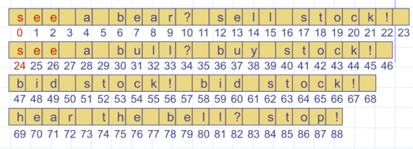
Word matching with a trie
- Insert words of the text into trie
- Each leaf is associated w/ one particular word
- Leaf stores indices where associated word begins (“see” starts at index 0 & 24, leaf for “see” stores those indices)
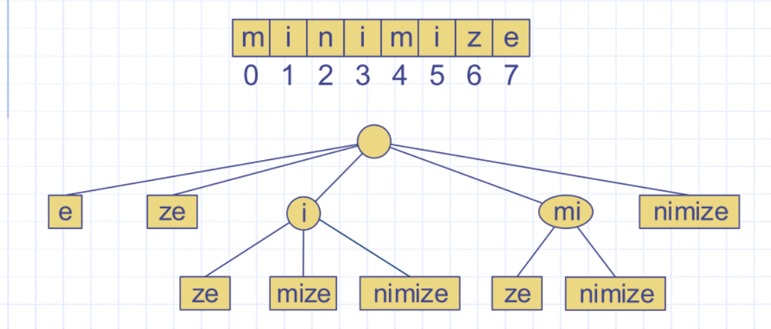
Compressed Tries
-
Compressed trie has internal nodes of degree at least two
-
Obtained from standard trie by compressing chains of redundant nodes
-
“i” and “d” in “bid” are redundant
- they signify the same word
- What is the maximum number of nodes in a compressed trie storing s words?
- s + (s -1) = 2 s -1
Compact Representation (NOT ON EXAM)
Want to create a compact representation of a compressed tree
Compact representation of a compressed trie for an array of strings
- Stores ranges of indices instead of substrings at the nodes
- Uses space, where s is the number of strings in the array
- Serves as an auxiliary index structure
Tries - outside of patterns
- Tries have other common uses outside of simple pattern matching (finding patterns in a given text efficiently)
- One common example: Autosuggestion engines
Input: Query Logs
- Take a large log of historical queries
- Count the number of times each query appears
- Basic idea: The autosuggestion engine should spit out suggestions based on historical popularity
- Input data then becomes a sequence of
pairs
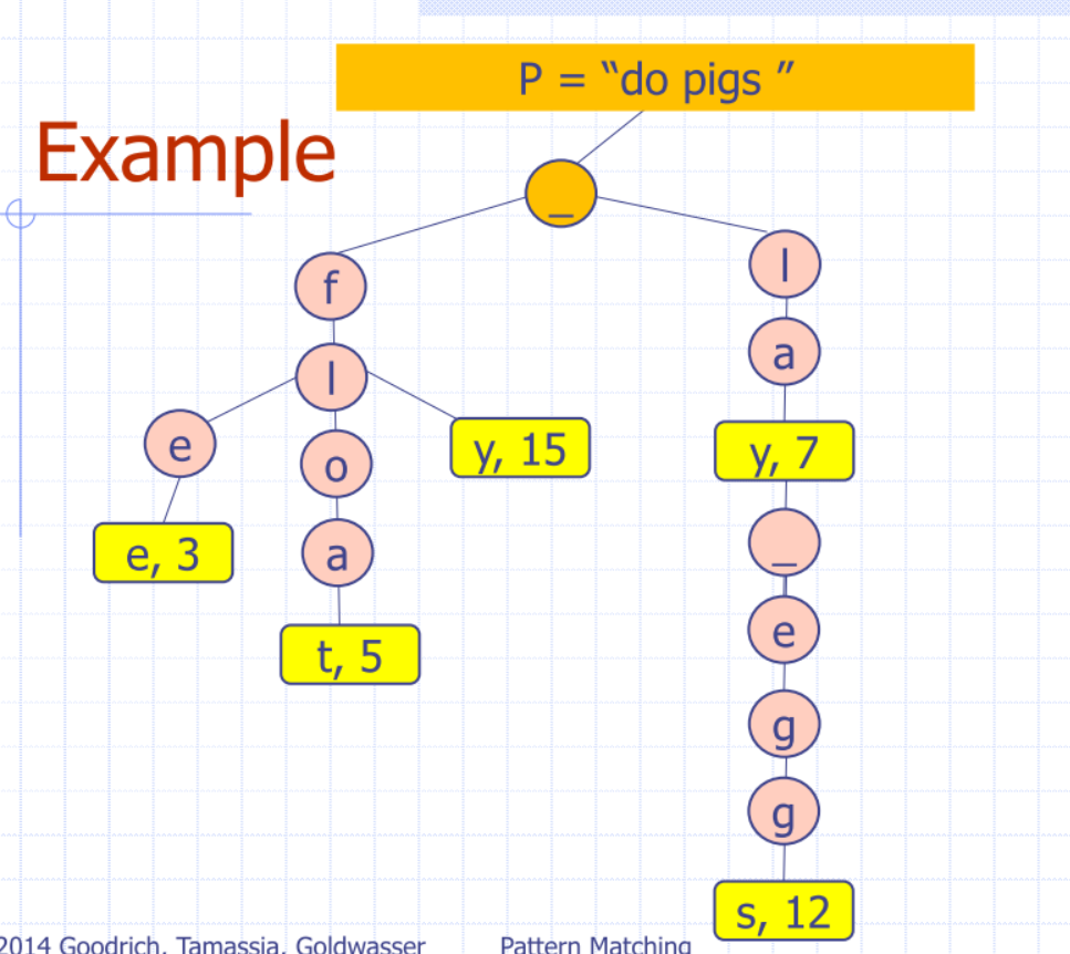
Building the Trie
- Each node (or edge) also holds a weight corresponding to the volume of queries that were issued for that prefix
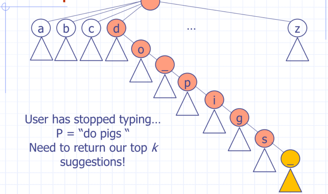
Querying the Trie
- Given a prefix P, we want to return a ranked list of k completions
- k is usually small, about 5-10 suggestions
- P is usually streamed, increasing in length
- Query starts empty, grows character-by-character
- Search is repeatedly triggered as the query is built, and suggestions returned ASAP!
- Only return endpoint suggestions – ranked by weight
| Given the prefix | return the list of k completions |
|---|---|
 |
 |
Suffix arrays
Suffix Tree (Suffix Trie)
- Suffix tree of a string
Tis the compressed trie of all the suffixes ofT
nsuffixes for a string of length n
Suffix Tree: Compact Rep.
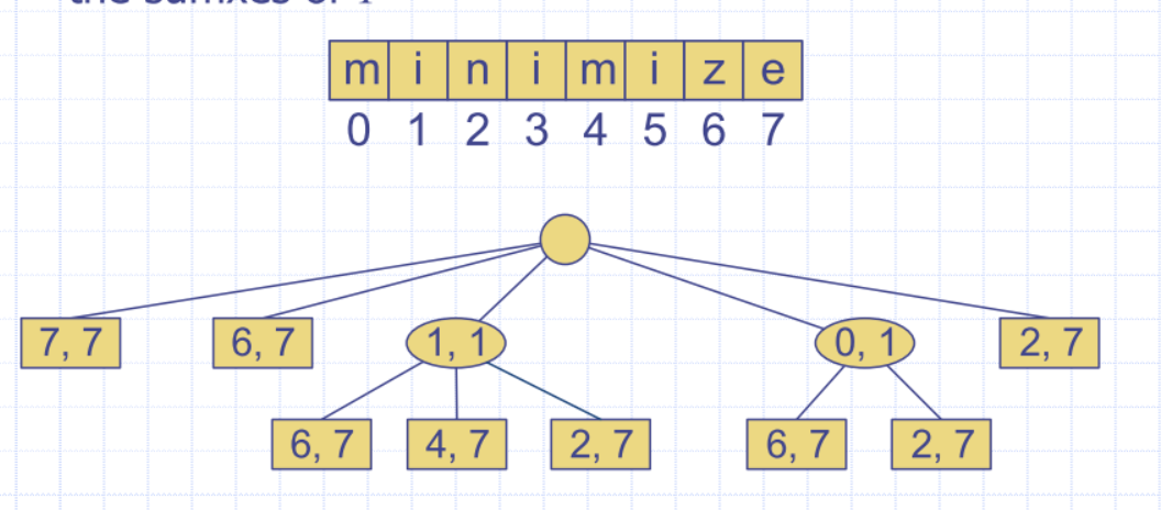
Suffix Tree Pattern Matching
- Maintain, at each node, the number of leaf nodes below
- Walk down the tree until we run out of pattern to match
- Return the count of leaf nodes below us
- find the patterns in text
- number of children in a suffix array
Other query types
- Count the number of occurrences of
PinT(we just saw this) - Output the locations of all occurrences of
PinT - Check whether
Pis a suffix ofT - Find the longest repeat in
T(the longest substring that occurs twice inT)
Given two strings A and B, what is their longest common substring?
- Idea: Create a new string by concatenating
AandBtogether with a special delimiterC = A|B(where ‘|’ is our special delimiter)
- Build a suffix tree on
C - Mark subtrees with a bit corresponding to whether the subtree holds a suffix of
A - Do the same for
B - The deepest node with both bits set is the longest common substring of both!
Analysis and performance
- Compact representation of the suffix tree for a string
Tof sizetfrom an alphabet of sized - Uses space (linear in the input text)
- Supports arbitrary pattern matching queries in
TinO(d x p)time, wherepis the size of the pattern- If we assume
disO(1), this becomesO(p)time - Then, finding all occurrences of P in T will cost
O(p + k)wherekis the number of timesPoccurs inT!
- If we assume
- Can construct a suffix tree in
O(t)time- Out of scope of this course: Ukkonen’s algorithm.
- If you have a text in a pattern, to find all positions of the pattern in the text, build a suffix tree and find them all much quicker
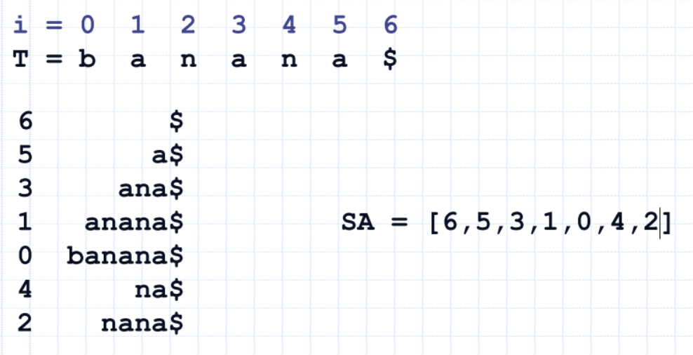
Suffix Arrays
-
Suffix Trees: Even though space consumption is
O(t)wheret = |T|(linear in the size of the indexed text), their pointer-based representation can be quite costly (Think about very large input strings…) -
Idea: We can use an array instead!
-
Write down all suffixes of T
-
The i-th suffix begins at position i
-
Sort the suffixes lexicographically, and let the i values “come along for the ride”
-
The resultant indexes are the suffix array!
Does the string “bana” occur in T ? Binary Search the SA!
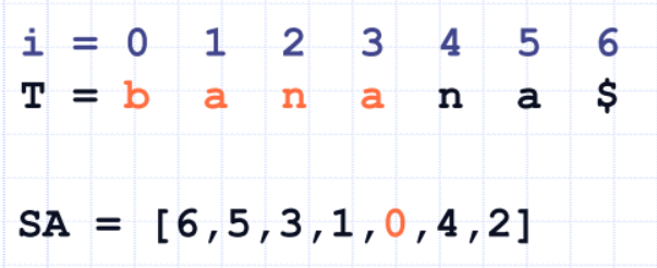
- MIGHT NEED LOWER BOUNDING
Suffix Array Analysis
- Can be constructed in linear time,
O(n)Out of scope for this course - Space occupancy is empirically better than the suffix tree (dont need to store pointers)
- Just store
Tand a list of integers!
- Just store
- May support a limited subset of suffix tree operations, but can be augmented to achieve more functionality