Lecture 3
Recap Lecture 2
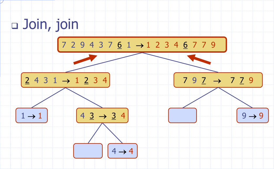
Quick-sort
- Randomised divide and conquer sorting algorithm
- Divide: pick a random element (called a pivot)
Quick sort recursion tree
- Execution of quick sort is depicted by a recursion tree
- Each node represents a recursive call of quick sort and stores
- Use the first element as a pivot, and divide the cards according to whether they are 'larger than' or 'smaller than' Good execution example:
The worst case running time
- The worst case occurs when picking the minimum or maximum element
Expected running time
- Good call: The size of and are each less than
- Bad call: one of or is greater than
Probabilistic fact: Expected number of coin tosses required in order to get heads is
In practise, quick sort is chosen over merge sort:
- Is in-place: only needs the array of data, no extra memory needed
- Keep track of pointers, and use them until they cross over
- In place partitioning - update textbook notes:
Sorting:
def bogo_sort(my_list):
    while is_sorted(my_list) == False:
        random_shuffle(my_list)
worst case: unbounded
Average case:
Best case:
Lecture 3
Counting Comparisons
- Each possible run of the algorithm corresponds to a root-to-leaf path in a decision tree
- If you traverse the tree, you can determine every element in relation to every other element's relation in the list
E.g. permutations
| permutation |
|---|
| a, b, c, |
| a, c, b |
| b, a, c |
| b, c, a |
| c, a, b, |
| c, b, a |
- Height of decision tree is a lower bound on running time
- Every unique input permutation must lead to a separate leaf
output
- if not, some input …4…5… would have same output ordering as …5…4…, which would be wrong
- There are leaves – height is at least
Every comparison based sort takes at best time
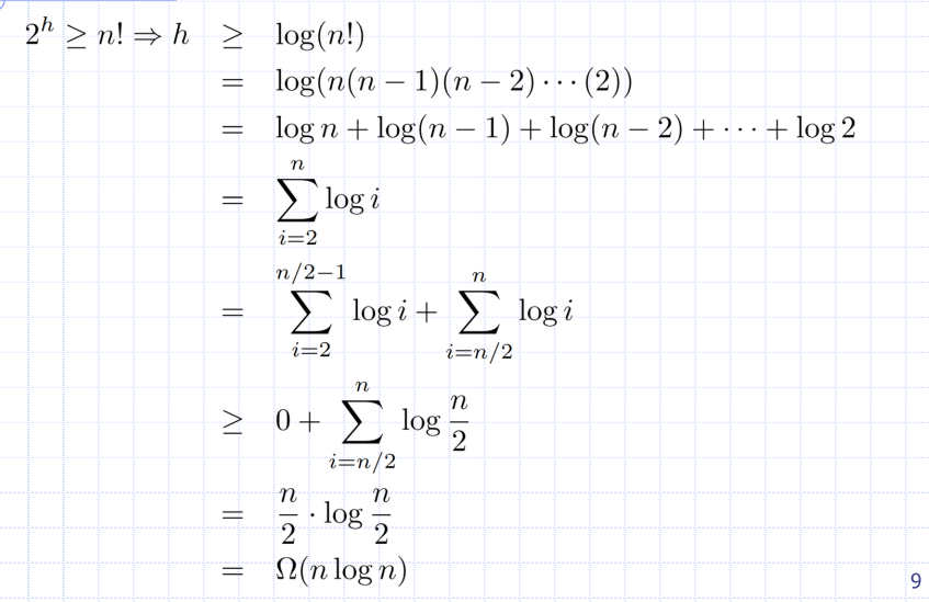
Lower Bound
- Comparison-based sorting algorithms takes at least log(n!) time
- ∴ any such algorithm takes at least
- Any comparison-based sorting algorithm must run in time
- merge and heap sorts are asymptotically optimal
- no other comparison sorts are faster by more than a constant factor
- merge and heap sorts are asymptotically optimal
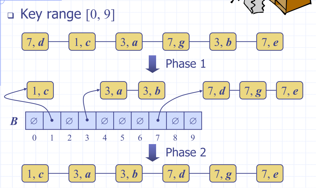
Bucket sort
- Let be a list of (key, element) items with keys in the range of [0, N-1]
- Create a bucket for each element
- Because the buckets are already sorted in the array, iterate through the buckets and link them together
Algorithm bucketSort(S):
  Input: sequence S of n entries with integer keys in the range [0, N − 1]
  Output: sequence S sorted in nondecreasing order of the keys

  B ← array of N empty sequences
  for each entry e in S do
    k ← key of e
    remove e from S
    insert e at the end of bucket B[k]
  for i ← 0 to N−1 do
    for each entry e in B[i] do
      remove e from B[i]
      insert e at the end of S
Analysis (algorithm above)
- Initialising the bucket array has to take time
- Phase 1 takes time
- Phase 2 takes time (has to iterate through each chain, in the whole bucket)
- Which ever of or will dominate depening on the size.
Properties and Extensions
- Stable sort property
- Relative order of any two items with the same key is preserved after the execution of the algorithm
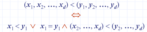
Lexicographic order:
- d-tuple is a sequence of d keys where key is said to be the i-th dimension of the tuple

Lexicographic-sort (Tuple sort)
- Comparator that compares two tuples by their dth dimension
- LexicographicSort sorts a sequence of d-tuples in lexicographic order by executing stableSort, d times
- Once per dimension
- Runs in time
- where is the running time of
stableSort
- where is the running time of
Algorithm lexicographicSort(S)
  Input sequence S of d-tuples
  Output sequence S sorted in lexicographic order
  for i <- d downto 1
    stableSort(S, Ci)
Radix sort
- Specialiation of lexicographic-sort
- Uses bucket sort as the stable sorting algorithm in each dimension
- Applicable to tuples where the keys in each dimension are integers in the range .
- Runs in time
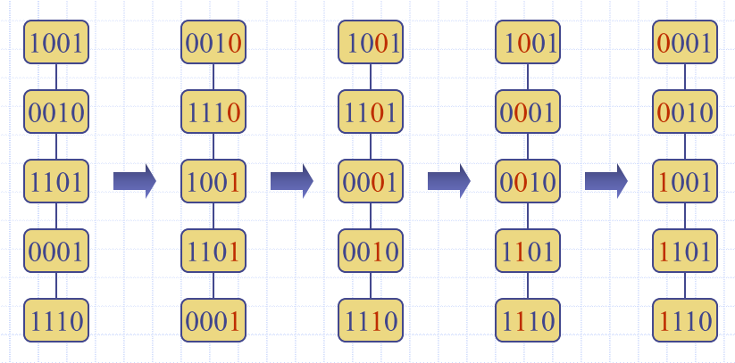
Radix-sort for binary numbers
- Consider a sequence of , -bit integers
- Represent each elements as a -tuple of integers in the range and apply radix-sort with
- Runs in or time. This is because we know N = 2
Example
Memory usage
- Original sequence and bucket array
- Sort: 10, 999, 3, 100,000,000, 20 Bucket Sort:
- (most will be empty)
Radix Sort: (converting to binary)
- space ovverhead is much more attractive
Arrays
A linear structure is one whose elements can be seen as being in a sequence. That is, one element follows the next.
- lists
- stacks
- queues
- Vectors
Static sequence ADT
ADT for a sequence: given a list of items in some order:
build(x): make new data stucture for items inlen(x): Return nget(x): return the element at position iset(i,x): set to x Arrays must be consecutive memory cells- size must be verified at creation (is static)
- constant random time access
- But what if we want to insert something?
- What if we need more space?
Dynamic Sequence ADT
- Same ADT as before, PLUS:
add(x)add to
Array implementation efficiency:
- Accessing an element
- Iterating over elements:
- Insert/Delete element:
- Memory Usage:
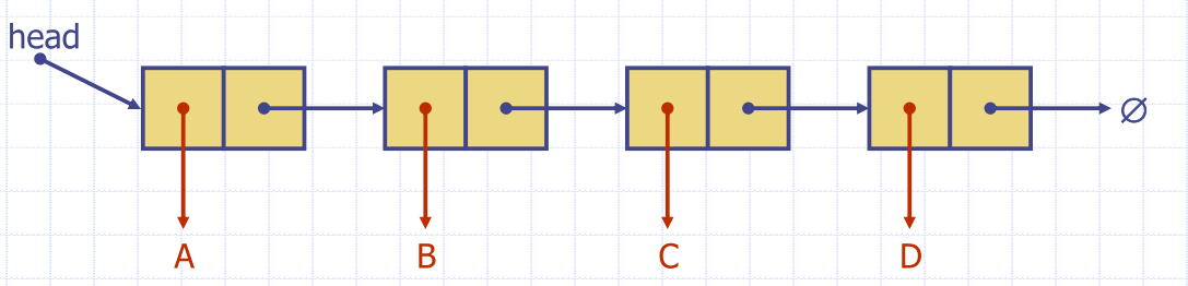
Singly linked list
- Concrete data structure
- sequence of nodes
- head pointer
- Nodes store
- element
- Link to next node
Simple process to insert between two elements
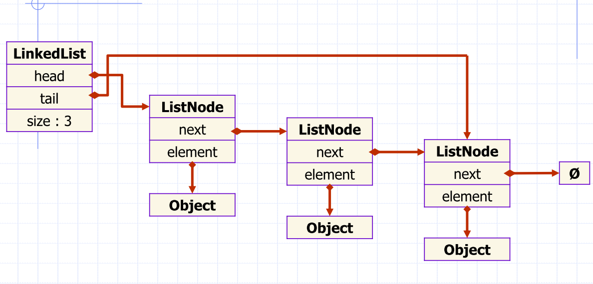
Singly linked list
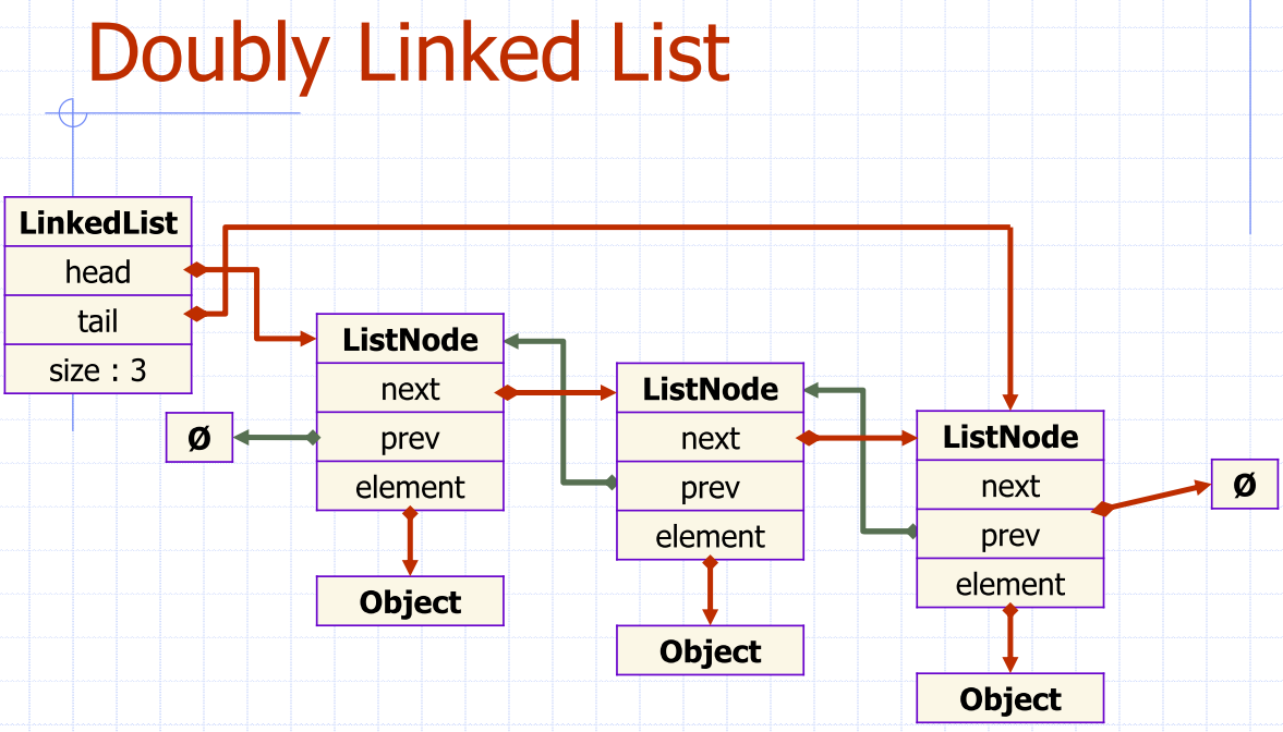
Doubly linked list
Circularly Linked list
Extensible lists
- push(o)/add(o)/append(o) adds element o at the end of the list
Linked list implementation efficiency
- Accessing an element
- Iterating over elements:
- Memory Usage:
- Insert/Delete element:
- Accessing tail
- Can do better by adding a reference to the tail
Note: Augmentation
- Accessing tail
class LinkedList:
  def __init__(self):
    self.__head = None
    self.__tail = None
    self.__size = 0
ExtensibleLists
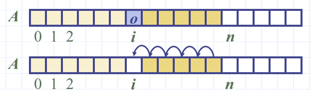
Insertion
- add(i, o) – make room for the new element
- Worst case (i = 0), takes O(n) time
Removal
- remove(i) – fill the hole left by the removed element
- Worst case (i = 0), takes O(n) time
Performance
- Array-based implementation of a dynamic list
- space used by the data structure is O(n)
- accessing the element at i takes O(1) time
- add and remove run in O(n) time
- add – when array is full
- instead of throwing an exception
- replace the array with a larger one
Extensible lists
- push(o)/add(o)/append(o) adds element
oat the end of the list - How large should the new array be if we run out of capacity?
- Incremental strategy
- increase size by a constant c
- double the size?
Comparison of Strategies
- Amortised time of a push operation is the average time taken by a push operation over the series of operations
Incremental strategy analysis
- a sequence of n pushes will take time per push
Doubling strategy analysis
- Array is replaced times
- Total time of of a series of push operations is proportional to
- Amortised time of push is