Lecture 9

Weighted Graphs

Each edge has an associated numerical value, called the weight of the edge
Edge weights may represent, distances, costs, etc.
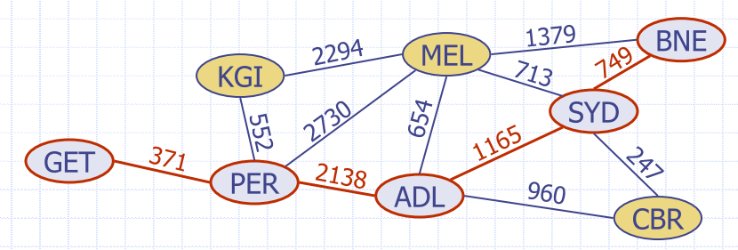
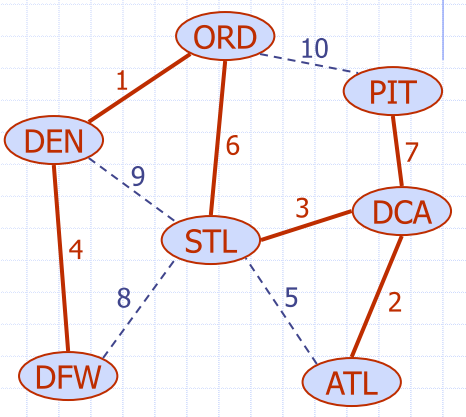
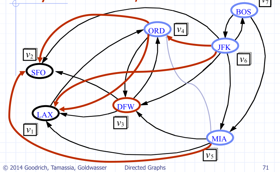
- e.g. flight route graph: weight of an edge represents the distance between the endpoint airports

Shortest Path

Given a weighted graph and two vertices u and v, find a path of minimum total weight between u and v
- length of a path is the sum of the weights of its edges
Example:
- shortest path between Brisbane and Geraldton

If every weight had the same cost

breadth first search would be the optimal algorithm

Alt text

Properties

Property 1:

Subpath of a shortest path is itself a shortest path Property 2:
There is a tree of shortest paths from a start vertex to all other vertices
- tree of shortest paths from Brisbane

You could have a single course of shortest path

E.g. the shortest path from brisbane, to any other airport

Dijkstra's Algorithm

Distance of a vertex v from a vertex s is the length of the shortest path between s and v
Dijkstra’s algorithm computes the distances of all the vertices from a given start vertex s
Assumptions
- graph is connected
- edges are undirected
- edge weights are not negative

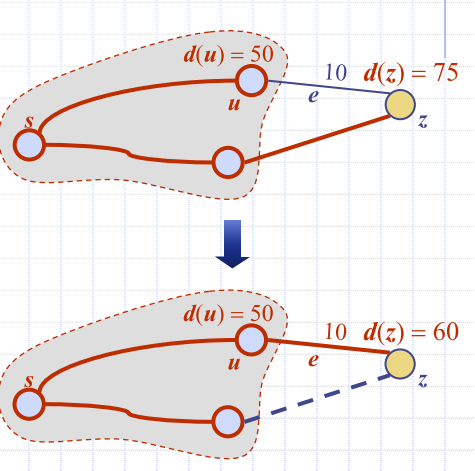
Edge relaxation

Consider an edge $e =(u, z)$ $e = (u, z)$ where
- u is the vertex most recently added to the cloud
- z is not in the cloud
Relaxation of edge e updates distance d(z)
- $d(z) \leftarrow min \; (d(z), d(u) + weight(e))$
Updating the label to be the shortest minimum distance
- iterative algorithm to traverse the vertex with the next shortest minimum weight

Dijkstra's Algoithm

Priority queue stores the vertices outside the cloud
- Key: distance
- Element: vertex
Locator-based methods
- insert(k, e) returns a locator
- replaceKey(l, k) changes the key of an item
Store two labels with each vertex
- Distance (d(v) label)
- locator in priority queue

Algorithm DijkstraDistances(G, s):
PQ <-new heap-based priority queue
for all  v <- G.vertices()
    if v = s
        setDistance(v, 0)
    else
        setDistance(v, (inf))
    PQ.insert(getDistance(v), v)
while !PQ.isEmpty()
    u <- PQ.removeMin()
    for all e in G.incidentEdges(u)
        { relax edge e }
        z <- G.opposite(u, e)
        r <- getDistance(u) + weight(e)
        if r < getDistance(z)
            setDistance(z, r)
            PQ.replaceKey(getLocator(z), r)

Analysis of Dijkstra's Algorithm

Graph operations
- find all the incident edges once for each vertex
Label operations
- set/get the distance and locator labels of vertex z $O(deg(z))$ times
- setting/getting a label takes O(1) time
Priority queue operations
- each vertex is inserted once into and removed once from the priority queue, where each insertion or removal takes $O(\log n)$ time ( $O(n \log n)$ changes total)
- key of a vertex in the priority queue is modified at most deg(w) times, where each key change takes $O(\log n)$ time (therefore $O(m \log n)$ key changes in PQ)
Dijkstra’s algorithm runs in $O((n + m) \log n)$ $O ((n + m) lo g n)$ time
- provided the graph is implemented as an adjacency list/map
- recall that $\sum_{v} deg(v) = 2m$
- can also be expressed as $O(m \log n)$ since the graph is connected

recall:

$n = |v|$ number of vertices
$m = |e|$ number of edges

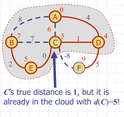
Why it Doesn’t Work for Negative-Weight Edges

Dijkstra’s algorithm is based on the greedy method

adds vertices by increasing distance
If a node with a negative incident edge were to be added late to the cloud, it could mess up distances for vertices already in the cloud.
- negative edges are going to 'mess up' distances already inside your cloud
- negative cycle - can keep on going around a cycle and costs keep getting lower and lower

Alt text

Greedy Algorithm

This that will benefit you the most, immediately from current point
best choice you can immediately at one point in time

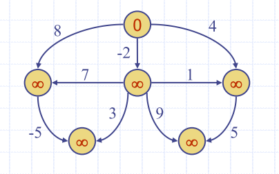
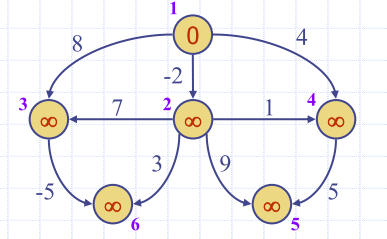
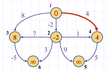
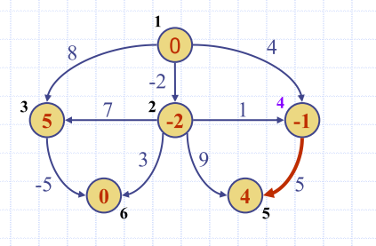
Dijkstra example

create a table to recount the edges of the shortest path

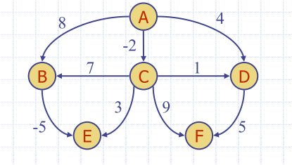
DAG-Based algorithm

Works even with negative-weight edges
Uses topological order
- Use topological order to iterate through all vertices, starting with the smallest topological ordering
Doesn’t use other data structures
Is much faster than Dijkstra’s algorithm
Running time
- O(n+m)

Algorithm DagDistances(G, s):
    for all  v <- G.vertices()
    if v = s
        setDistance(v, 0)
    else
        setDistance(v, )
    { Perform a topological sort of the vertices }
    for u <- 1 to n do    {in topological order}
        for each  e <- G.outEdges(u)
            { relax edge e }
            z <- G.opposite(u, e)
            r <- getDistance(u) + weight(e)
            if r < getDistance(z)
                setDistance(z, r)

init	Label nodes with initial distances	Topological sort	visit in topological order	result

Downside of DAG Approach?

Not all graphs are DAG's

Minimum Spanning trees

Spanning Subgraph
- subgraph of a graph G containing all vertices of G
Spanning Tree
- spanning subgraph that is itself a (free) tree
Minimum Spanning Tree (MST)
- spanning tree of a weighted graph with minimum total edge weight

Alt text

Aren't MST's = shortest path?

We know that single-source shortest path yields a trwee of shortest paths from origin u
Can we just run that?
- No
Minimum spanning tress might not exactly the same as the shortest path - if the node we're starting from has high weights

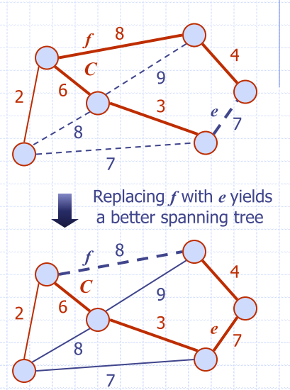
Cycle property

Let T be a MST of a weighted graph G
Let e be an edge of G that is not in T
Let C be the cycle formed by e with T
For every edge f of C, weight(f) $\le$ weight(e)

Alt text

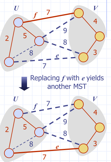
Partition Property

Consider a partition of the vertices of G into subsets U and V
Let e be an edge of minimum weight across the partition
There is a minimum spanning tree of G containing edge e

Proof

Let T be an MST of G
If T does not contain e, consider the cycle C formed by e with T and let f be an edge of C across the partition
By the cycle property, weight(f) $\le$ weight(e)
Thus, weight(f) = weight(e)
We obtain another MST by replacing f with e

Alt text

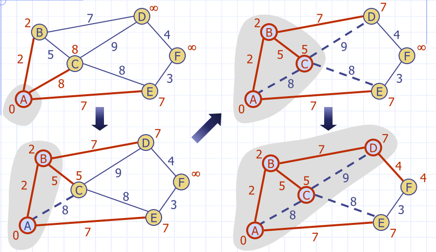
Prim-Jarnik’s Algorithm

Similar to Dijkstra’s algorithm
Pick an arbitrary vertex s and grow the MST as a cloud of vertices, starting from s
Store with each vertex v, a label d(v)
- smallest weight of an edge connecting v to a vertex in the cloud
At each step
- add to the cloud the vertex u outside the cloud with the smallest distance label
- update the labels of the vertices adjacent to u

KEY DIFFERENCE: Not trying to find the minimum distance, trying to find the minimum spanning tree

Alt text

Analysis

Graph operations
- cycle through the incident edges once for each vertex
Label operations
- set/get distance, parent and locator labels of vertex z O(deg(z)) times
- setting/getting a label takes $O(1)$ time
Priority queue operations
- each vertex is inserted once into and removed once from the priority queue, where each insertion or removal takes $O(\log n)$ time
- key of a vertex w in the priority queue is modified at most deg(w) times, where each key change takes $O(\log n)$ time
Prim-Jarnik’s algorithm runs in $O((n + m) \log n)$ $O ((n + m) lo g n)$ time
- provided the graph is represented by an adjacency list structure
- recall that $\sum_{v} deg(v) = 2m$
- can also be expressed as O(m log n) since the graph is connected

Recall:

$n = |v|$ number of vertices
$m = |e|$ number of edges

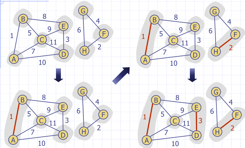
Kruskal's Approach

Maintain a partition of the vertices into clusters
- initially, single-vertex clusters
- keep an MST for each cluster
- merge “closest” clusters and their MSTs
Priority queue stores the edges outside clusters
- key: weight
- element: edge
At the end of the algorithm
- one cluster and one MST

Algorithm Kruskal(G)
    Input: a simple connected weighted graph G with n vertices and m edges
    Output: a minimum spanning tree T for G

for each vertex v in G do
    define an elementary cluster C(v) = {v}
Initialise a priority queue Q to contain all edges in G, using the weights as keys
T -> null           {T will ultimately contain the edges of the MST}

while T has fewer than n-1 edges to
    (u,v) = value returned by Q.remove_min() (``find``)
    Let C(u) be the cluster containing u, and let C(v) be the cluster containing v
    if C(u) != C(v) then
      add edge (u,v) to T
      Merge C(u) and C(v) into one cluster (``union``)
return tree T

Alt text

Data Structure for Krukal's Approach

Algorithm maintains a forest of trees
Priority queue extracts the edges by increasing weight
An edge is accepted if it connects distinct trees
Need a data structure that maintains a partition, i.e., a collection of disjoint sets, with operations:
- makeSet(u): create a set containing new element u
- find(u): return the set storing u
- union(A, B): replace sets A and B with their union

List-based partition

Each set is stored in a sequence
Each element has a reference back to the set
- find(u) takes $O(1)$ $O (1)$ time, and returns the set of which u is a member
  - Ackuman function (grows far worse than exponential)
  - actually grows the inverse of the Ackuman function $O(\alpha (n))$
- union(A, B) moves the elements of the smaller set to the sequence of the larger set and updates their references
  - takes $min(|A|, |B|)$ time
Whenever an element is processed, it goes into a set of size at least double, hence each element is processed at most $log n$ times

Partition-base implementation

Partition-based version of Kruskal’s Algorithm
- cluster merges as unions
- cluster locations as finds
Running time of kruskal's algorithm: $O((n + m) \log n)$ $O ((n + m) lo g n)$
- priority queue operations: $O(m \log n)$ $O (m lo g n)$
  - Is actually $O(m \log m)$ but we note that $m$ is $O(n^{2})$ for a simple graph. Using log laws we get to this result.
- union-find operations: $O(n \log n)$ $O (n lo g n)$
  - each position can be charged at most $O(\log n)$ times, since the size of the cluster's group doubles each time. Occurs max $n$ times, therefore, $O(n \log n)$

Solving Graph problems

Single Pair Reachability:
- Is there a path from $u$ to $v$ in $G$ ?
Single Pair Shortest Path:
- What is the shortest path (and its cost) from $u$ to $v$ in $G$ ?
Single Source Shortest Path:
- What is the shortest path (and associated costs) from v to all other u in G?
All-Pairs Shortest Paths:
- What is the shortest path (and associated costs) between all pairs of vertices in G?
Each problem is at least as hard as the previous one…
- Use properties of your specific problem to help solve it. Is the graph a DAG? Are the weights always positive? …

Extension Material

NONE OF THIS WILL APPEAR ON THE FINAL EXAM

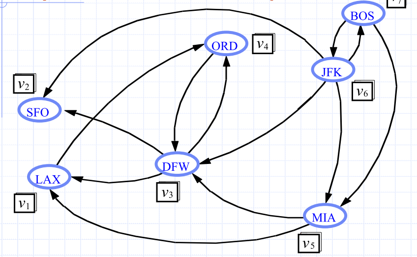
Transitive Closure

Given a digraph G, the transitive closure of G is the digraph G* such that
- G* has the same vertices as G
- if G has a directed path from u to v (u $\ne$ v), G* has a directed edge from u to v
Transitive closure provides reachability information about a digraph

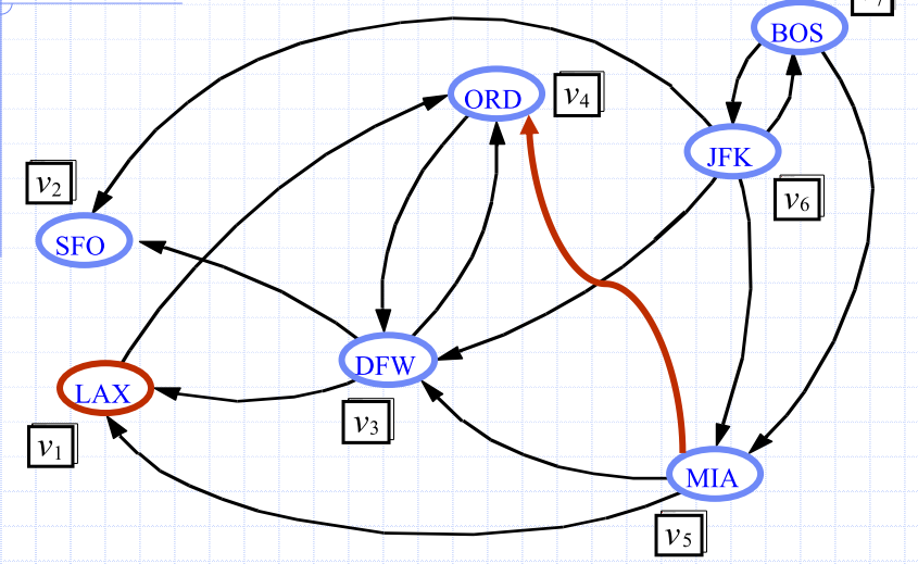
Computing Transitive Closure

Perform DFS starting at each vertex
- O(n(n+m))

Dynamic Programming

Powerful technique for solving problems
Idea: Break the problem into smaller subproblems
- Solve the subproblems
- Combine the solutions to solve the full problem
- Reuse subproblem solutions (only compute once, cache the result)

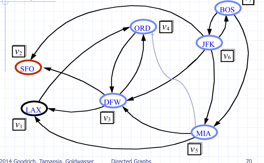
Floyd-Warshall Algorithm

Number vertices $v_{1}, ..., v_{n}$
Compute Graphs $G_{0}m ..., G_{n}$ $G_{0} m ..., G_{n}$
- $G_{0} = G$
- $G_{k}$ has directed edge $(v_{i}, v_{j})$ if $G$ has a directed path from $v_{i}$ to $v_{j}$ , with intermediate vertices $v_{1}, ..., v_{k}$
$G_{n} = G^{*}$
In phase $k$ , digraph $G_{k}$ is computed from $G_{k-1}$
Running time: $O(n^{3})$ assuming areAdjacent is $O(1)$ e.g. adjacency matrix

iteration 0	iteration 1	iteration 2	iteration 3

All pairs shortest paths

Floyd-Warshall can also be used to solve the All-Pairs Shortest Path problem
Can handle directed, weighted graphs, even where weights are negative!
Cannot handle negative cycles a cycle in a graph where the weights summed up is less than 0
But it may be modified to detect them
Bellman-Ford can detect negative cycles, but solves SSSP, not APSP
Johnson’s algorithm can solve APSP in any weighted graph
- Can detect negative cycles

Joels insights:

Weighted or not?
- Weights positive or not?
Directed or undirected?
Simple?
- Self loops or parallel edges?
Cycles? Negative cycles?