Chapt 3.1. Experimental studies

We are interested in the desgin of "good" data structures and algorithms

Data Structure: a systematic way of organising and accessing data

Algorithm: A step-by-step procedure for performing some task in a finite amount of time.

Experimental studies

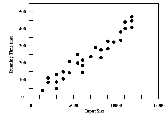
We can study the running time of an algorithm by recording the time spent between each execution

for time import time
start_time = time()
# run the algorithm
end_time = time()
elaqpsed = end time - start_time

We can use this approach to gather experimental data on the efficiency of Python's list class
Not the best measure of algorithm efficiency; other background process may yield and unfair test. A fairer metric is the number of CPU cycles that are used by the algorithm

We are interested in the general dependence of running time on the size and structure of the input.

Perform independent experiments on many different test inputs of various sizes, i.e.

Challenges of experimental analysis:

Experimental running times of two differing algorithms are difficult to compare unless experiements are performed on the same hardware and software requirements
Experiments can only be completed on a limited set of inputs
An algorithm must be fully implemented in order to execute it, to study its running time experimentally.

Goal of experimental analysis:

Evaluate relative efficiency of algorithms in a way that is independent of the hardware and software envrionment
Is performed at a high-level description of the algorithm without need for implementation
Takes into account all possible inputs.

Counting prime operations:

Perform an analysis directly on a high-level description of the algorithm. Define a set of primitive operations such as the following:

Assigning an identifier to an object
Determining the object associated with an identifier
Performing an arithmetic operation (e.g. adding two numbers) A primitive operation corresponds to a low-level instruction with an execution time that is constant.

Henceforth, to capture the growth of an algorithms's running time, we will associate a function $f(n)$ that characterises the number of primitive operations performed, relative to the input size $n$ .

Focus on worst-case input

characterise the running times in terms of the wrost case, as a function of the input size, $n$ , of the algorithm.
- easier than avergae case analysis

Recursion

Begin with the following four example of the use of recursion, providing an python implementation for each:

The factorial function
An English rules
Binary search
File system for a computer, in which directories can be nested arbitrarily deep within other directories

The factorial function

n! = \begin{cases} 1 & \text{if } x \in n = 0\\ n \cdot (n-1)\cdot (n-1) \cdot \cdot \cdot 2 \cdot 1 & \text{if } x \ge 1 \end{cases}

There is a natural recursive definition for the factorial function. Observe that $5!=5\cdot 4 \cdot 3 \cdot 2 \cdot 1 = 5\cdot 4!$ . Thus, the recrusive defintion can be formalised as

n! = \begin{cases} 1 & \text{if } x \in n = 0\\ n \cdot (n-1)! & \text{if } x \ge 1 \end{cases}

Recursive implementation of the Factorial function

def factorial(n):
    if n == 1:
        return 1
    else:
        return n * factorial(n-1)

repetition is provided by the repeated invocations of the function

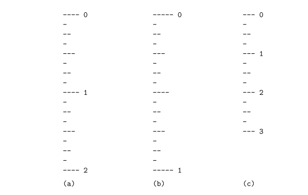
Drawing the English Rulers

For each inch, we place a tick with a numeric label. We denote the length of the tick designating a whole inch as the major tick length
Between marks for whole inches, the rules contains a series of minor ticks, placed at intervals of 1/2 inch, 1/4 inch, etc.

Although it is possible to draw such a ruler with iteration, the task is considerably easier with iteration

Python Implementation

def draw_line(tick_length, tick_label=''):
"""Draw one line with given tick length (followed by optional label)"""
line = '-' * tick_length
if tick_label:
    line += ' ' + tick_label

def draw_interval(center_length):
    """ Draw tick length based upon a central tick length."""
    if center_length > 0:       # stop when length drops to 0
        draw_interval(center_length - 1)    # recursively draw top ticks
        draw_line(center_length)            # draw center tick
        draw_interval(center_length - 1)    # recursively draw bottom ticks

def draw_ruler(num_inches, major length):
    """Draw English ruler with given numbr of inches, major tick length"""
    draw_line(major_length, '0')        # draw 0 inch line
    for j in range(1, 1+num_inches):
        draw_interval(major_length - 1)     # draw interior tick for inch
        draw_line(major_length, str(j))     # draw in j line and label

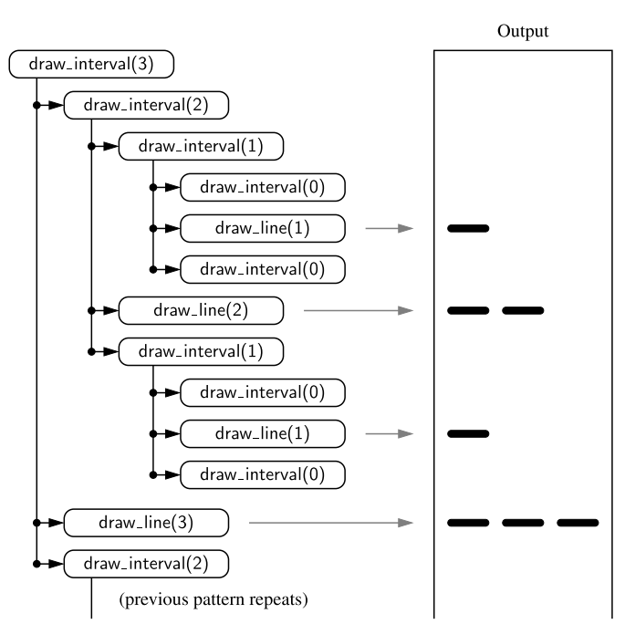
The execution of the recursive draw_interval function can be visualised using a recursion trace.

Binary search

This algorithm is used to efficiently locate a target value within a sorted sequence of $n$ elements.

When the standard sequence is unsorted, the standard approach is to use a loop to examine every element, until either finding a target or exhausting a dataset
When sorted and indexable, we know that the values stored at indices $0,...,j-1$ are less than or equal to the value at index $j$ -> same for values greater than $j$ .
- The algorithm maintains two parameters, low and high, such that all the candidate entries have index at least low and at most high.
  - Initially, low = 0 and high = $n-1$
  - compare the target value with the median candidate $mid=\lfloor(low+high)/2\rfloor$
Consider three cases:

If the target equals data[mid], return the result
If target < data[mid], recur the first half of the sequence
If target > data[mid], then recur the second half of the sequence

Whereas a sequential search runs in $O(n)$ time, binary search runs in $O(\log n)$ time

""" Return true us target is found in indicated portion of a Python list
The search only considers the portion from data[low] to data[high] inclusive
"""
def binary_search(data, target, low, high):
    if low > high:
        return False
    else:
        mid = (low+ high) // 2
        if target == data[mid]:
            #recur on the portion left of the middle
            return binary_search(data, target, low, mid-1)
        else:
            #recur on the portion right of the middle
            return binary search(data, target, mid + 1, high)

File Systems

A file system consists of a top-level directory, and the contents of this directory consists of files and other directories, which in turn contain files and other directories, and so on. The operating system allow directories to be nested arbitrarily deep

Many common behaviours of an operating system, such as copying a directory or deleting a directory are implemented as recursive algorithms
The cumulative disk space for an entry can be computed with a simple recursive algorithm

Algorithm DiskUsage(path):
    Input: A string designating a path to a file-system entry
    Output: The cumulative disk space used by that entry and any nested entries
    total = size(path)
    if path represents a directory then
        for each child stored within directory path do
            total = total + DiskUsage(child)
    return total

Analysing Recursive Algorithms

For each recursive algorithm, we will account for each operation that is performed based upon the particular Activation of the function that manages the flow of control at the time it is executed

i.e. only account for the number of operations that are performed within the body of that activation
Can then account for the overall number of operations that are executed as part of the recursive algorithm
- This can achieved by understanding the recursion trace of each algorithm

Factorial algorithm

To compute factorial(n), we see there are a total of $n+1$ activations, as the parameter decreases from n in the first call, to $n-1$ , etc.
Therefore, the overall number of operations computing factorial(n) is $O(n)$

Drawing an English ruler

Consider how many lines of input are generated by an initial call to draw_interval(c)
We know that a call to draw_interval(c) for $c>0$ spawns two calls to draw_interval(c-1) and a single call to draw_line.
For all $c \ge 0$ , a call to draw_interval(c) results in precisely $2^{c} - 1$ lines of output
- More generally, the number of lines priented by draw_interval(c) is one more than twice the number generated to call draw_interval(c-1)

Performing a Binary Search

The running time of a binary search algorithm is proportional to the number of recursive calls performed
The binary search algorithm runs in $O(\log n)$ times for a sorted sequence with $n$ elements
- Initially, the number of candidates is $n$ , after the first call in a binary search, it is at most $n/2$ ; after the second call $n/4$ ; and so on. In general, after the $j$ th call in a binary search, the number of candidate entries remaining is at most $n/2^{j}$ .

Recursion run Amok

An inefficent recursion for Computing Fibonacci Numbers

Fibonacci:

F_{0} = 0

F_{1} = 1

F_{n} = F_{n-2} + F_{n-1}, n>1

A direct implementation based on the algorithm would be as follows:

def bad_fibonacci(n):
    """Return the nth Fibonacci number"""
    if n <= 1:
        return n
    else:
        return bad_fibonacci(n-1) + bad_fibonacci(n-2)

Computing the fibonacci sequence depends on the two previous values $F_{n-1}$ and $F_{n-2}$ , but the call to compute $F_{n-1}$ requires it's own recursive call to compute $F_{n-2}$ -> does not have the knowledge of that value

Computing the nth Fibonacci number in this way requires an exponential number of calls to the function. The number of calls $c_{n}$ for input size $n$ is $c_{n}>2^{n/2}$ , which mean that bad_fibonacci(n) makes a number of calls that is exponential in $n$ .

We can compute $F_{n}$ much more efficiently in which invocation only makes one recursive call. Rather than having the function return a single value, we define a recursive function that returns a pair of consecutive fibonacci numbers.

def good_fibonacci(n):
    """ Return pair of Fibonacci numbers, F(n) and F(n-1)"""
    if n <= 1:
        return (n, 0)
    else:
        (a, b) = good_fibonacci(n-1)
        return (a+b, a)

The execution of good_fibonacci(n) table $O(n)$ time.

4.4 Further examples of Recursion

If a recursive call starts at most one other, we call this linear recursion
If a recursive call starts two others, we call this binary recursion
If a recursive call starts more than two others, we call this Multiple recursion

Linear recursion

Implementation of factorial function and good_fibonacci function are examples of linear recursion
Note that linear recursion reflects the structure of the recursion trace, not the asymptotic analysis of the running time

Example: Summing the elements of a sequence recursively

The following computes the sum of a sequence

def linear_sum(S, n)
""" Compute the sum of a sequence of the first n numbers of Sequence S"""
    if n == 0:
        return 0
    else:
        return linear_sum(S, n-1) + S[n-1]

Binary recursion

Revisit the problem of summing $n$ elements of s sequence $S$ , of numbers. With two or more elements, we can recursively compute the sum of the first half, and the sum of the second half, and ad these together as shown in the following:

def binary_sum(S, start, stop):
    """ Return the sum of the numbers in implicit slice S[start:stop]. """
    if start >= stop:
        return 0
    elif start == stop - 1:
        return S[start]
        else: 
            mid = (start + stop) // 2
            return binary_sum(S, start, mid) + binary_sum(S, mid, stop)

The size of the range is divided in half for each recursive call, and uses $\log n$ amount of additional space, compared to $n$ space used in the linear_sum function. However, the running time of binary_sum is $O(n)$ , as there are $2n-1$ function calls, each requiring constant time.

Multiple recursion

The recursion of analysing the disk space usage of a file system is an example of multiple recursion, because the number of recursive calls made during one invocation was equal to the number of entries within a given directory of a file system.

Designing Recursive algorithms

An algorithm that uses recursion typically has the following form:

Test for base cases. Begin by testing for a set of base cases (there should be at least one)
Recur. If not a base case, we perform one or more recursive calls. This may involve a step that decides which of several possible recursive calls to make.

Eliminating tail recursion

Some forms of recursion can be eliminated without any use of auxillary memory. A notable form is known as tail recursion.

A recursion is a tail recursion if any recursive call that is made from one context is the very last operation in that context, with the return value of that recursion immediately returned by the enclosing recursion.
Of the recursive functions demonstrated in this chapter, the binary_search and reverse function are examples of recursion.
Any tail recursion can be reimplemented nonrecursively by enclosing the body in a loop for repition, and replacing a recursive call with new parameters by a reassignment of the existing parameters to those values.

def binary_search(data, target):
    """return True if target is found in the given python list"""
    low = 0
    high = len(data) - 1
    while low <= high:
        mid = low+high // 2
        if target == data[mid]:
            return True
        elif target < data[mid]:
            high = mid - 1
        else:
            low = mid + 1
    return False

Where we made a recursive call binary_search(data, target, low, mid-1) in the original version, we replace high = mid - 1 in our new version and continue our iteration.