Lecture 12

• Basel - regulations about how a bank regulates it balance sheet
• central metrics are VaR and ES to measure market risk that a bank has
• Bank regulation protects depositor funds
  • Most people cannot assess the creditworthiness of a bank, basel regulations protect depositors

Risk concepts

We first discuss some basic concepts relating to risk, which we use later:

• What is risk?
• Individual security risk.
• The normal distribution.
• Portfolio risk.

FINM3405 is titled “Derivative securities and risk management” and we’ve discussed some hedging concepts in an “ad hoc” fashion.

• But what do we really mean by “risk” and “risk management”?

Define risk as the dependence of a portfolio’s or a company’s value, solvency, or profits, etc, on external factors that are unpredictable and out of the control of the portfolio or business manager.

Derivative securities are tools in larger toolkits used in more general risk management frameworks within businesses and fi nancial institutions, which involves the identification, measurement and control of risks.

• Involved in the identification of risk and the exposure of risk
• VaR is the expected shortfall and quantifying it

Types of Risks

We could classify risk into the following 4 broad categories:

1. Market risks: These are the risks we’ve mostly been discussing this semester, namely risks due to movements in market variables such as interest rates, exchange rates, stock prices, commodity prices, etc.
2. Liquidity risk: The inability to sell or liquidate assets and financial securities quickly and at prices close to fair market values.
3. Credit risk: The risk of loss due to borrowers and counterparties failing to meet, and thus defaulting on, their payment obligations.
4. Operational risks: “All others” including human error, fraud and theft, model risk, technology failure, legal risk, weather events, etc.

Of course these categories are not “water tight”.

• Market risk, risks are due to move in financial market variables, prices, interest rates, economic growth
  • Concerned mostly about this.
  • Have a market/trading portfolio, exposed to price movements/exchange rate movements
• Liquidity risk - inability to liquidate out of a position quickly in the market
  • Property - pretty illiquid relative to shares
• Credit risk - can't meet their obligations in a timely manner
  • meeting payment obligations
  • Default risk - worried that the counterparty may not meet their obligations
    • Typically trade with a dealer though
• Operational risk
  • everything else - technology failure, electricity may go off, legal risks, etc.
  • Security returns are normally distributed - not realistic in real life

• This semester we’ve discussed using derivative securities to control or manage (hedge against) various sources of risk we may face.
• We also discussed ways of measuring or quantifying market risks:
  • Standard deviation σ (volatility) and beta β (systematic risk).
  • Delta ∆, gamma Γ, vega ν, rho ρ, theta θ of options positions.
• We also discussed survival probabilities, loss given default and recovery rates, probability of default, etc, which are ways of measuring and quantifying to credit risk.
• You may also recall the notions of duration and convexity for interest rate securities and portfolios, particularly bonds.

• beta, systematic risk between portfolio and market
• Why VaR and ES are important

There is a very large range of individual risk measures, metrics and techniques for quantifying diff erent kinds of market, liquidity and credit risk, including and not limited to those mentioned above.

• Furthermore, financial institutions will hold a very large number and variety of positions across all asset classes, from stocks, interest rates, currencies, loans, derivatives, property, etc - you name it.
• And financial institutions will individually measure and quantify in the best way they can all the risks they face across all their positions using all available metrics and techniques specific to their positions.

Consequently, you could imagine that the situation would get quite complicated and complex, with all these diff erent traders and departments in a big bank all measuring their unique exposures and risks in their own unique ways relating to the particular positions they hold.

• However, managers, the board of directors, regulators, etc, require simple to understand and simple to calculate measures of “aggregate” or “institution-wide” or “total” risk.
• In other words, they want a fi nancial institution’s risks “all packaged up” into single, simple to understand metrics or measures.

Value at risk (VaR) and expected shortfall (ES) seek to do this for a bank’s market risks: package them all up into a single total risk measure.

• Big financial institutions, all different positions in different securities
  • unique to particular financial instruments
  • Use the large variety of risk metrics, where the individual risk measures are unique to the asset class
• All different positions, hard to compare risk between financial instruments
• Management are not going to know what these risk metrics are going to mean
  • Need simple to understand risk metrics

Individual security risk

We first refresh some introductory calculations about individual security and portfolio risk or volatility (standard deviation) which we use later.

• Let $\{R_1 , . . . , R_N\}$ be $N$ time period returns for a financial asset.

Recall that the mean return is given by

$$\mu = \frac{1}{N} \sum ^N _{i=1} R_i$$

Also recall that the volatility (standard deviation) in returns is

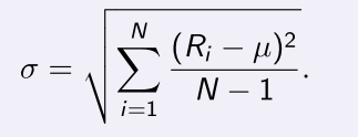
• sigma is called an unbiased estimator

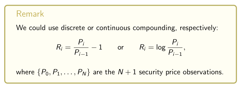
How do we calculate returns?

Later, we’ll also use some notions relating to the normal distribution:

Normal distribution

If we’re willing to believe that returns are normally distributed (and we will make this dubious assumption later) then the mean µ and variance σ 2 completely characterise the probability distribution of the returns:

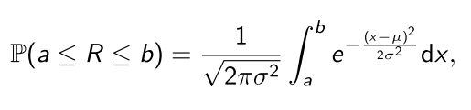
where $R$ is the random variable representing the security’s returns.

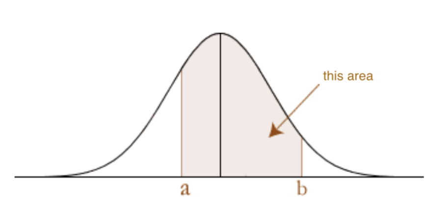
• In words, $P (a ≤ R ≤ b)$ is the probability of the asset’s returns $R$ falling between a and b, that is, in the interval $[a, b]$.
• It is the area under the normal distribution PDF over [a, b], namely:

under the standard normal PDF

Later we will use the normal distribution to model the distribution of changes dV in the value V of a portfolio.

• And here, we’re mostly interested in the “left tail” probabilities:

• When it comes to VaR and ES, we are concerned about the left tail probabilities

The CDF of the standard normal distribution (µ = 0 and σ 2 = 1) is

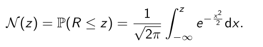
For negative z-values, it gives the following “left tail” area or probability:

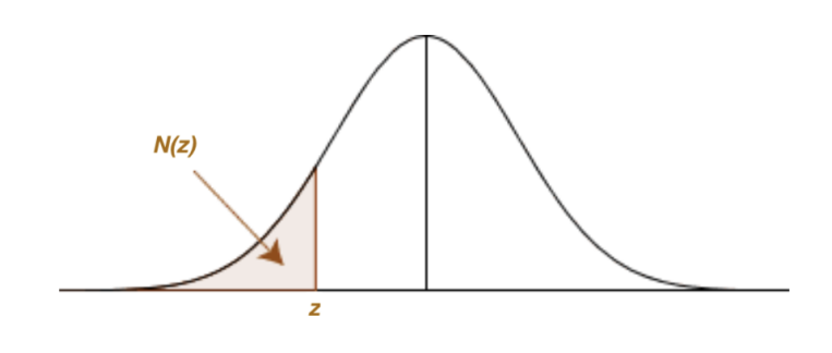
We will also denote these “left tail” areas or probabilities α = N (z).

• Quantifying the probability of losses on a trading book
• Probability of earning a loss, is given by a cdf
  • If we are working with a normal distribution
• use $\alpha$ for the area in the tail
  • also use p values
• losses worse than or equal to a given loss,
• What is the loss we would receive 5% of the time

Later, when doing VaR and ES calculations, we’re interested in the following “left tail” areas α = N (z) and z-values z that give them:

• $α = N (−1.645) = 0.05.$
• $α = N (−1.96) = 0.025.$
• $α = N (−2.326) = 0.01.$

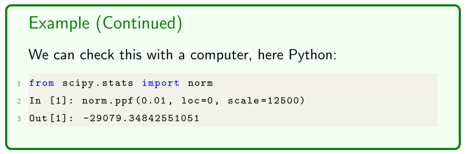
We can find these z-values using norm.ppf() in Python:

1 from scipy . stats import norm
2 In [1]: norm.ppf (0.05)
3 Out [1]: -1.6448536269514729
4 In [1]: norm.ppf (0.025)
5 Out [1]: -1.9599639845400545
6 In [1]: norm.ppf (0.01)
7 Out [1]: -2.3263478740408408

Above we’re using the standard normal distribution, which has a mean of $µ = 0$ and variance of $σ^2 = 1$. But what about for a general normal distribution with non-zero mean µ and variance $σ^2$ different to 1?

• To find the z-value $z_α$ corresponding to a given left tail probability or area α for a normal distribution with mean µ and variance $σ^2$ we set

$$z_α = µ + zσ$$

where z is the z-value for a standard normal distribution corresponding to the left tail probability $α = N (z)$

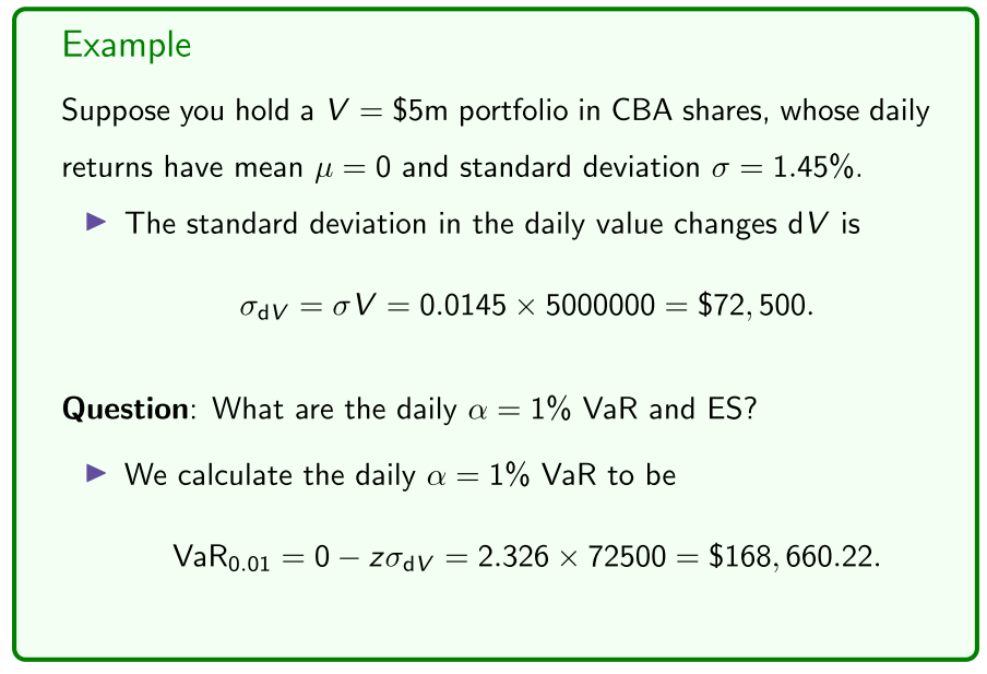
Example

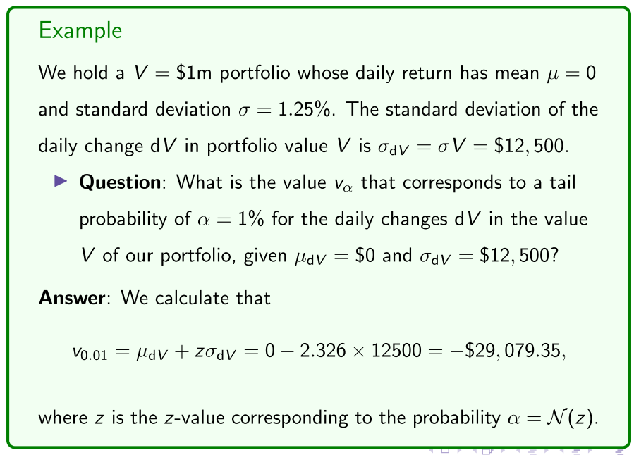
• typical z value for the normal distribution

Remark

We note upfront that when doing value at risk (VaR) and expected shortfall (ES) calculations, we’re interested in the time period (say daily) changes dV in the portfolio value V , which we think of as dollar value profits/losses over the given time period.

• interested in the dollar value changes in a portfolio

Portfolio risk

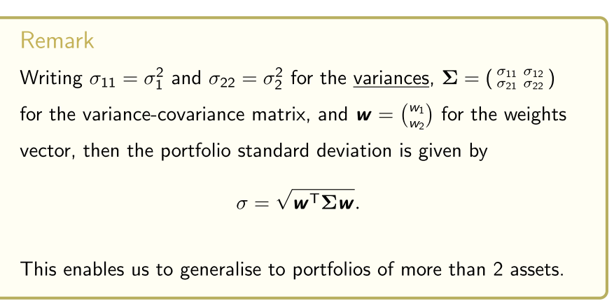
We now refresh calculating portfolio return means and volatilities: Suppose we hold a portfolio of 2 assets with mean returns $µ_1$ and $µ_2$, and standard deviations (volatilities) in returns $σ_1$ and $σ_2$. If we have $w_1$ and $w_2$ weights (percent) invested in asset 1 and 2, then we recall that:

• Our portfolio mean return is

$$µ = w_1 µ_1 + w_2 µ_2$$

• Our portfolio standard deviation in returns is

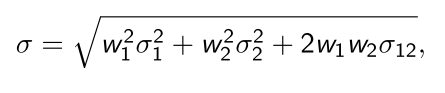
with $σ_{12} = σ_1 σ_2 ρ$ and $ρ$ the covariance and correlation in returns.

VaR and ES

Using tail probability $α = 1 − p$, value at risk (VaR) answers:

What is the maximum dollar loss $VaR_α$ that would be incurred over a given time period with probability p?

Ie: “We will lose at most $VaR α over the time period in p% of cases.”

• From the “opposite” perspective:

What is the minimum dollar loss VaR α that would be incurred over a given time period with probability α? Ie: “We will lose at least $VaR α over the time period in α% of cases.”

• What is the most we can lose
  • Tail probability,
• 1-p, other side, area to the right side, level or confidence
  • What are the bad outcomes we are risking of losing
  • maximum amount we can lose with 99% confidence?

Minimum loss we could occur

• There is a 1% chance of losing the value of risk, or even more
• maximum loss at a given probability

For some terminology and notation:

• VaR α is the value at risk (what we risk losing).
  • It’s the most we’d lose with probability $p = 1 − α$
  • Or the least we’d lose with probability $α = 1 − p$.
• $p$ is the level of confidence.
  • It’s typically set to p = 95%, or p = 97.5%, or p = 99%.
• $α = 1 − p$ is called the tail probability.
  • It’s typically small at α = 5%, α = 2.5%, α = 1%, etc.
• Also, the time period is usually “small” at 1 or 10 days.

$VaR_α$ is possibly best conceptualised graphically:

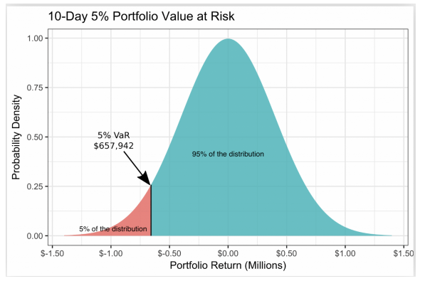
This is the distribution of a portfolio’s value changes dV over a 10-day period.

The α = 5% VaR is VaR 0.05 = $657, 942, which in words is:

• VaR 0.05 is the worst outcome over 10 days with p = 95% confidence.
• Or, α = 5% of the time we lose at least VaR 0.05 dollars over 10 days.

• 95% confident they are going to to lose at most 657,000

Remark

In other words, using the previous notation, $VaR_α$ is the negative of the value $v_α$ corresponding to a left tail probability of α%.

So we can “rephrase” the previous example:

Example

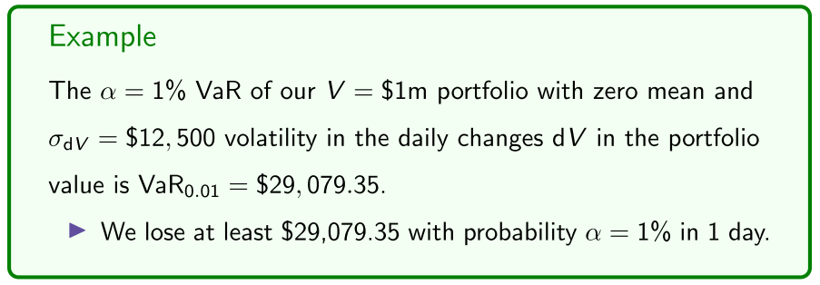
Remark

$VaR_α$ tells us the least amount we expect to lose with tail probability α% in a given time period.

So VaR has the shortcoming that it does not tell us what our expected tail risk or loss or shortfall (ES) is, that is, how much we expect to lose if our portfolio outcomes fall in the α% left tail area of the distribution.

• Two distributions may have the same VaR α but different expected losses or shortfalls $ES_α$ for a given left tail probability α, as in:

• May have the same VaR point, but the expected amount to lose might be very different

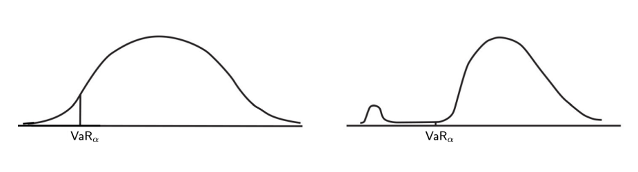
• Expected loss we are going to incur might be a lot worse
• regulators moved from VaR to Expected shortfall

Both distributions have the same VaR $α$ but you expect larger losses (much larger than $VaR_α$) in the RHS distribution than the LHS, if the outcomes fell in the α% left tail area of the distribution (left of $VaR_α$).

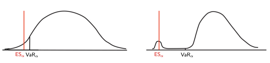
• The expected shortfall (ES) answers the question:

How much $ES_α$ do we expect to lose if our outcomes fall in the α% left tail area of the distribution, so to the left of $VaR_α$?

Probabilistically, $ES_α$ is the expected value or mean in the case that our outcomes are worse than (left of) $VaR_α$ for a given tail probability α:

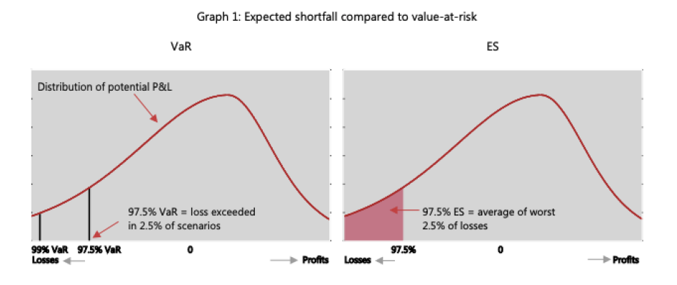
Remark

Regulators use $VaR_α$ and $ES_α$ to calculate the amount of capital a bank needs to hold to remain solvent: $≥ 3 × ES_α$ I believe.

From the Bank for International Settlements’ Explanatory note on the minimum capital requirements for market risk:

Question: Given tail probability α, how do we calculate $VaR_α$ and $ES_α$ ?

VaR and ES estimation methods

We cover two contrasting approaches to VaR α and ES α calculation:

1. Parametric: Assumes the distribution of changes dV in our portfolio value V can be described or modelled by a known “parametric family” of probability distributions.

• We assume the normal distribution.
• Uses historical data to estimate the parameters µ and $σ^2$ of the best fitting normal distribution to calculate $VaR_α$ and $ES_α$.

2. Nonparametric: We don’t assume a “parametric family”, but instead use historical data directly to construct histograms and “rank” or “order” or manually “sort” the changes dV in our portfolio value V in order to calculate VaR α and ES α for a given α. We start with the parametric method:

Parametric

• slightly more complicated formula
• assuming that the probability distributions of the returns are modelled by a probability distribution

Non-parametric

• financial data is not normally distrbuted
• historical returns of profit outcomes, and rank from loss to best profit, and pick the 1% of the worst outcomes

Parametric

When asset returns are normally distributed with mean µ and variance $σ^2$, for a given left tail probability α we already know that the value at risk $VaR_α$ of the change dV in the portfolio value V is given by

$$VaR α = −(µ_{dV} + zσ_{dV} )$$

with z the z-value of the standard normal distribution corresponding to the left tail probability $α = N (z)$. The expected shortfall $ES_α$ is

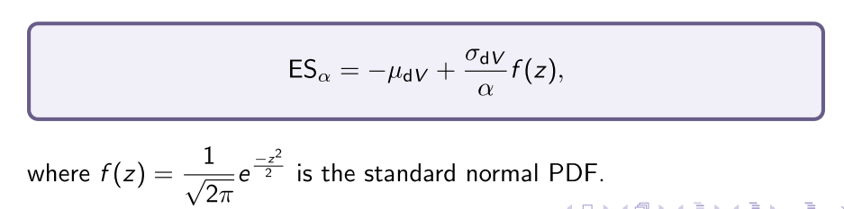
Example

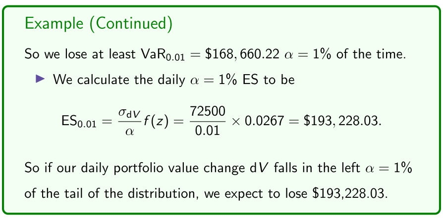
• lose at least this 1% of the time
• lose at most this 99% of the time

Sanity check - ES to be higher (worse) the VaR

Parametric portfolio VaR

We now want to write the portfolio VaR α in terms of the values at risk $VaR_{α,1}$ and $VaR_{α,2}$ of asset 1 and 2 in the portfolio:

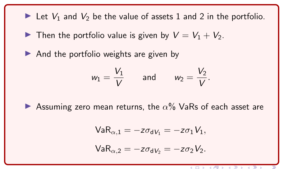
• deriving (red box)
• standard deviation of the returns multiplied by the first asset
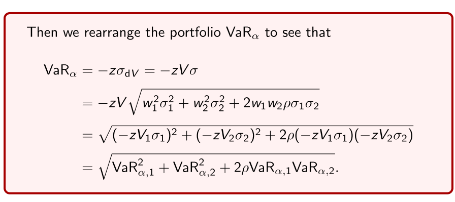
• portfolio VaR - use Markowitz formla
  • do a bit of rearranging,

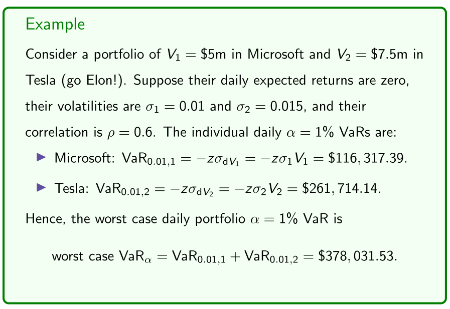
The result we want to remember is the portfolio $VaR_α$ is given by

Question: Do we get portfolio $VaR_α$ diversification benefits?

Answer: Yes provided that the assets are not perfectly correlated.

• First observe that when ρ = 1 (perfect correlation), we get

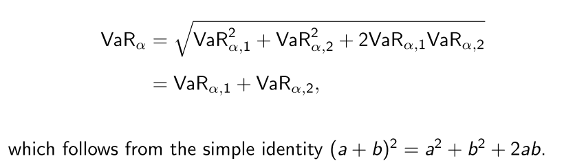
The worst case portfolio $VaR_α$ is thus defined as

$$worst case VaR_α = VaR_{α,1} + VaR_{α,2}$$

It represents no $VaR_α$ diversification benefits due to perfect correlation.

So the worst case portfolio $VaR_α$ is when the assets are perfectly correlated (ρ = 1), and is just the sum of the individual VaRs.

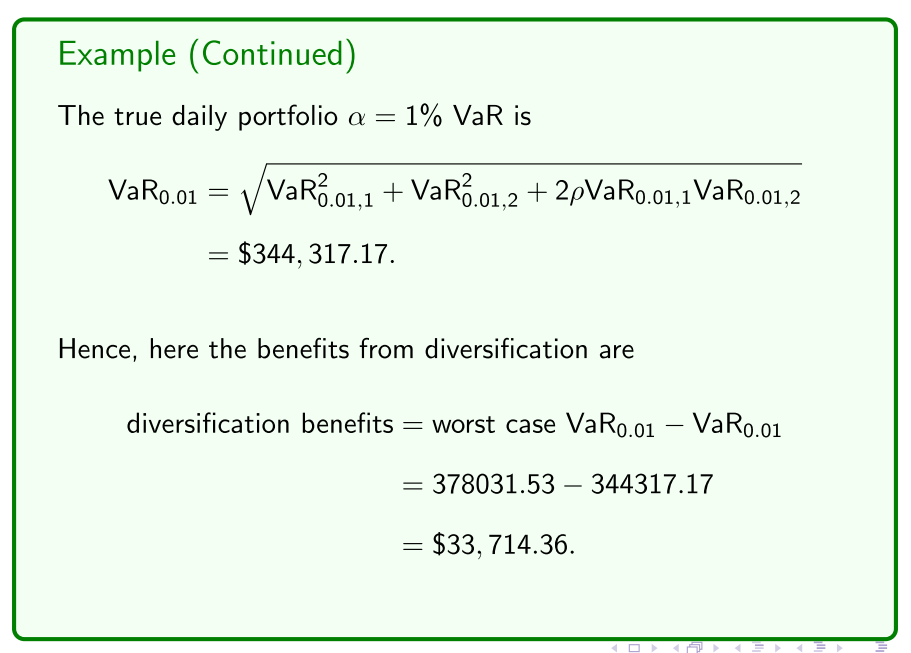
• From the portfolio $VaR_α$ formula, when ρ < 1, the portfolio $VaR_α$ is less than the worst case $VaR_α$.

We define the benefits from diversification to be

Example

IN FINAL EXAM

Nonparametric

But wait, there’s just one problem with the above parametric method:

• Financial asset returns are not normally distributed!

Consequently, we could consider fitting a different family of distributions to asset returns, such as a Student’s t-distribution, which even has a closed-form solution for the expected shortfall:

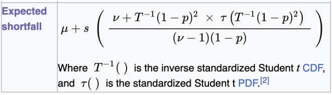
Here µ is the mean, s is the standard deviation, ν is the degrees of freedom, τ and T are defi ned in the image, and p is the level of confi dence as above, so1 − p is the tail probability. But we don’t do this.

• t-distribution does have a closed form
• not going to do this

We present the nonparametric (historical simulation) method for estimating $VaR_α$ and $ES_α$, as follows:

• Collect a sample $\{P_0 , P_1 , . . . , P_N \}$ of N + 1 historical asset prices.
• Calculate the historical returns $\{R_1 , . . . , R_N \}$ given by

$$R_i = \frac{P_i}{P_{i-1}} - 1 \;\;\; \text{or} R_{i} = \log{P_i}{P_i-1} \;\; \text{for} i=1,...N$$

Now suppose we hold a portfolio of Q units in the (single) asset whose current price is P. The current portfolio value is therefore

$$V = QP$$

Using the returns sample $\{R_1 , . . . , R_N\}$, we get a sample $\{dV 1 , . . . , dV_N\}$ of portfolio value changes starting at the current value $V = QP$ given by

$$dV_i = VR_i \text{for} \;\; i = 1, . . . , N$$

We can then plot a histogram of the portfolio value changes $\{dV 1 , . . . , dV_N\}$ to visually inspect the distribution.

• And we calculate the VaR α and ES α as follows:

• Get a sample of daily value changes
• Sample of daily value changes, is our distribution of value changes
• plot a histogram and order daily value changes
• visually inspect the histogram and calculate the average of the expected shortfall
  • most ways regulators do it
  • other more complicated approaches

To calculate the VaR α and ES α we order or rank the portfolio value changes dV i from smallest to largest (largest loss to largest profi t):

• By definition, the α% VaR is the portfolio value change dV i that leaves α% of the portfolio value changes “to the left” of it.
• Also, by definition the α% ES is the average (or mean) of these α% portfolio value changes that are “to the left” of VaR α .

• alpha % is the actual individual portfolio

Remark

Due to the sample size N, there may not be a portfolio value change dV i that leaves exactly α% of the portfolio value changes to the left of it, so VaR α and ES α will be slight, but usually quite accurate, approximations, which improve as N increases.

Example

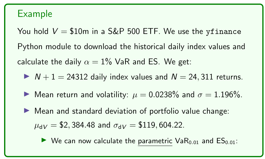
• goes up on average 2384 per day

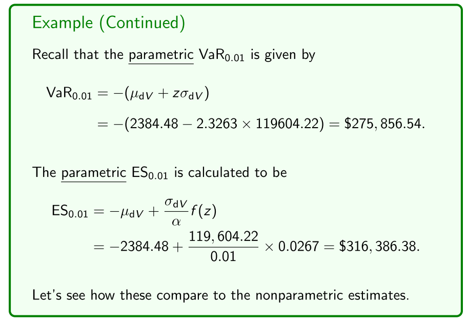
• going to lose at least 275000 1% of the time

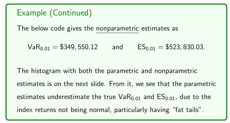
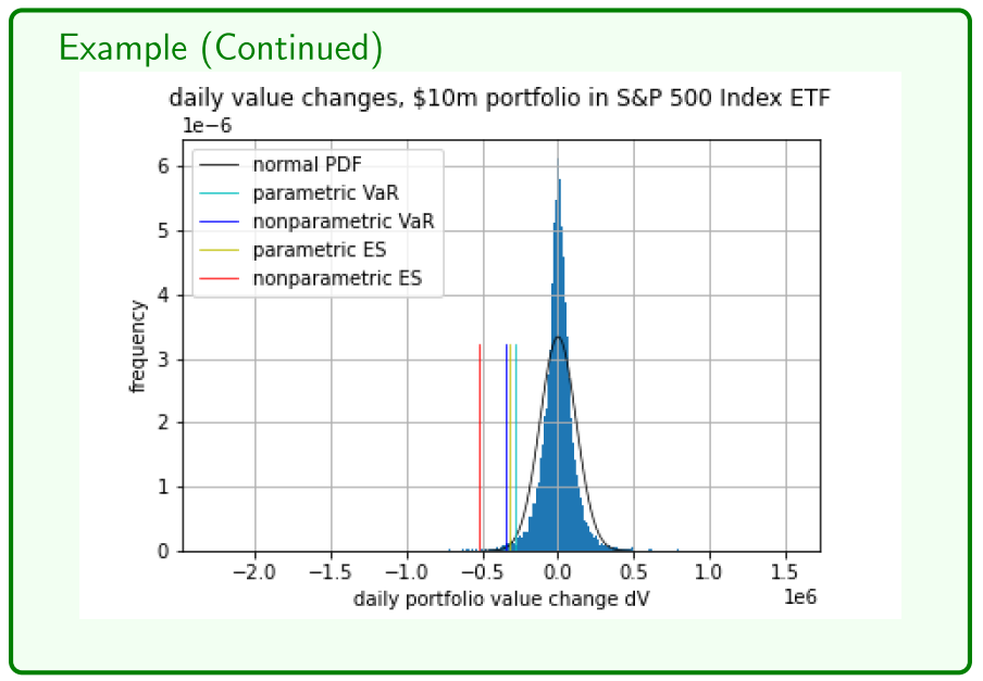
• non-parametric shortfall is a lot worse
• fit another distribution that would model it more accurately