Lecture 3

Readings: Chapters 3 and 5 of Hull.

Last week we saw that at the time of writing, the S&P 500 spot price was 5,633.91, but the CME Group E-Mini futures September contract price was 5,682.5 and the December contract price was 5,748.

• This week we cover futures pricing, which means calculating the theoretically correct contract prices.
• We also cover optimal hedging, since most hedging scenarios in practice are rarely as “neat and clean” as those from last week.

Why is there a discrepancy in the future price vs the spot index price?

• December contract, even greater

Contract pricing

Recall that the value at time $t$ of a long futures or forward position entered into at an earlier time $t = 0$ is

$$V^{long}_{t} = e^{-r(T-t)}\cdot (K_{t}-K)$$

Pricing a futures or forward contract at time $t$ involves using no-arbitrage arguments to calculate the contract price $K_{t}$ that yields $0$ value to short and long positions entered into at time $t$.

• close out initial long position at some time $t$
• short position, contracting the close the position at $K_{t}$
• maturity date is capital T

Value to the short and long party is $0$ at time $t$

Remark: The time $t$ at which we price contracts is arbitrary so in what follows we simply let $t = 0$ in order to reduce notation, and in which case there is $T$ years to maturity or the delivery date.

• Initially bought and closed the position, the value of the position would equal $0$ (last term in the equation would cancel out)
• Always imagine time is $t=0$. Now is the current date $t$, $T$ is the delivery/expiry date

General Notation

• We work on a hypothetical time interval $[0, T]$.
  • Time $t = 0$ is the date we enter into a contract.
  • Time $T$ is a contract’s maturity or delivery date.
  • Time $t$ is some intermediate date: $0 ≤ t ≤ T$.
• $S_{t}$ is the underlying asset’s spot price at time t.
• $K_{t}$ is the contract price at time t.
  • We write $S = S_{0}$ and $K = K_{0}$ to reduce notation.
• $m$ is the number of assets in 1 contract (the multiplier).
• $h$ is the number of contracts we enter into.

Cost Of Carry Notation

In order to present the basic cost-of-carry arbitrage argument for pricing futures and forwards, we use the following additional notation:

• $I$ is the time $T$ capitalised interest paid on a loan used to buy the underlying asset at time $t = 0$.
• $J$ is the time $T$ capitalised storage cost of owning and holding the underlying asset from time $t = 0$ to time T.
  • Transport, warehouse storage, insurance, maintenance, etc.
• $D$ is the time $T$ capitalised dividends or other income or benefits received from owning the asset up to time T.
  • Share dividends, foreign interest, convenience/benefit from holding the asset in stock and/or using or consuming it, etc.

• wheat, corn, some kind of commodity might need to be insured or stored
  • need to spend money maintaining the asset
  • J - capitalised storage costs
  • from time t=0 to T at regular intervals. Compound them forward to the maturity date. E.g. multiple interest payments that are made
    • Put all the intermediate payments to one date.

Income

• Any incomes we might receive for owning the asset
  • Dividends, e.g.
  • Might receive multiple payments, compounded forward to the maturity date (that is why it is called capitalised)

Remark: By “time T capitalised” we mean that any cashflows (loan or coupon payments, storage costs, dividends or other income, etc) received or paid between times $t = 0$ and $T$ are capitalised or compounded forward to time $T$.

$$K = S + I + J − D$$

Arbitrage: transactions

To show why K = S + I + J − D must hold, consider the following arbitrage arguments:

Suppose $K > S + I + J − D$ and consider the following short trade: Transactions at time t = 0:

• Borrow $S$ to buy 1 unit of the underlying asset spot.
• Short 1 contract to sell the asset for $K$ at maturity $T$.

Note that your net cashflow at time $t = 0$ is 0, since the money you received from borrowing was used to buy the asset.

Transactions at maturity, time T:

• Receive K for selling the asset in the contract.
• Pay off the loan S with interest I.
• Pay J for owning, holding and storing the asset.
• Receive any other income D from owning the asset.

Then your net cashflow at maturity is positive:

$$K − S − I − J + D > 0$$

Keep borrowing to buy the asset and short the contract for no initial net cashflow, but receive the positive net cashflow at maturity: An arbitrage.

Remark Another way to look at it is in terms of contract value. If $K > S + I + J − D$ then your short trade locks in the positive cashflow of $K − S − I − J + D$ at maturity.

• This cashflow is thus risk free and its value

$$V^{short} = e^{-rT}\cdot (K-S-I-J+ D) > 0$$

is positive to you and negative to the long position.

• You’d need to compensate the long position by this amount. But K is set so the contract has 0 initial value to both parties.

Not thinking about counterparty risk at this stage

• credit risk - other party won't honor their obligations
• call it risk free at this stage

Arbitrage: transactions cont

Also, if $K < S + J + I − D$ and if you currently own the underlying asset, then you can consider taking the following long position:

Transactions at time $t = 0$:

• Sell the asset spot for $S$ and invest the proceeds.
• Go long to buy back the asset for $K$ at maturity $T$.

Transactions at maturity, time $T$:

• Pay $K$ for buying back the asset in the contract.
• Receive $S$ plus interest $I$ from investing.
• Receive (more accurately, not have to pay) $J$ for no longer having to own, hold and store the asset.
• Pay (more accurately, no longer receive) any other income $D$ from no longer owning the asset.

Then your net cashflow at maturity is positive since

$$-K+S+I+J-D>0$$

Remark: Again, your net cashflow at initiation is 0.

$$V^{long} = e^{-rT}\cdot (-k+S+I+J-D) > 0$$

which represents negative value to the short party who would demand this amount in compensation upfront or they wouldn’t be interested in entering into the contract.

Have to pay the short party to enter into the contract

Cost of Carry

We thus get the cost of carry model for pricing forwards and futures:

$$K = S + I + J − D$$

Here $I + J − D$ is the net cost of carrying (holding, storing) the asset.

Remark

The cost of carry model is usually written with annual borrowing rates $r$, storage rates $s$ and dividend or convenience yields $q$, and is called spot-forward parity since it defines the relation between spot and forward prices

• normally written in terms of borrowing rates
• normally called spot forward parody

Let

• $r$ be a simple annual interest rate,
• $s$ be a simple annual storage rate, and
• $q$ be a simple annual dividend (or later convenience) yield.

Then the cost of carrying the asset is

$$I + J − D = SrT + SsT − SqT.$$

• The cost of carry relation $K = S + I + J − D$ becomes

$$K = S[1 + (r + s − q)T]$$

and is called spot-forward parity. Under compound interest it becomes

Simple interest

$$K = S(1 + r + s − q)^{T}$$

or (Compound Interest)

$$K = Se^{(r+s−q)T}$$

What is the relation between spot S and forward K prices?

From:

$$K = Se^{(r+s−q)T}$$

if the cost of carry $r + s − q$ (in rates) is:

• Positive, so $r + s − q > 0$ then $K > S$ (forward prices are greater than spot prices) and we say the market is normal.
• Negative, so $r + s − q < 0$ then $K < S$ (forward prices are less than spot prices) and we say the market is inverted.

Commodity contract pricing

In the case of commodity futures and forwards, we have the:

• Interest rate $r$ on borrowing and lending.
• Carrying cost $s$ representing storage and insurance, etc, costs.
• Convenience yield $q$ representing benefits of owning the asset:
  • Wholesalers maintain adequate stock levels to supply their customers in a timely and reliable manner.
  • Manufacturers maintain adequate stock in order to use/consume and keep their production processes running and not get held up.

So the cost-of-carry model and spot-forward parity relation is as above.

• People are willing to pay a premium to have stock in inventory
• Receive an abstract benefit for keeping their supplies in stock
  • Quantified in commodity futures
• Cost of carry model

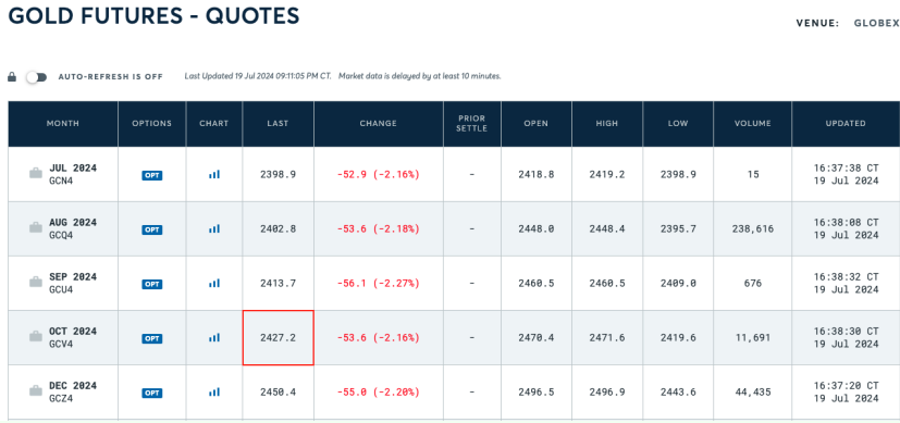
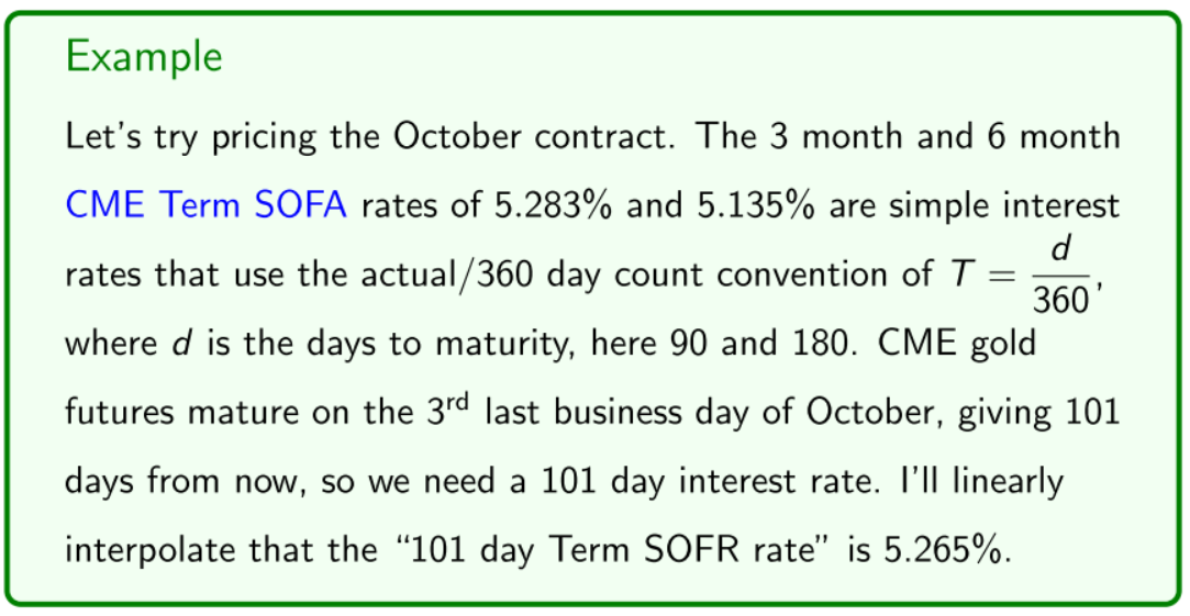
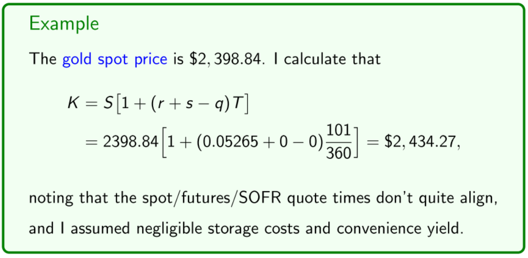
CME Gold futures contract

Gold Futures Quotes	Spot Price	interest rates
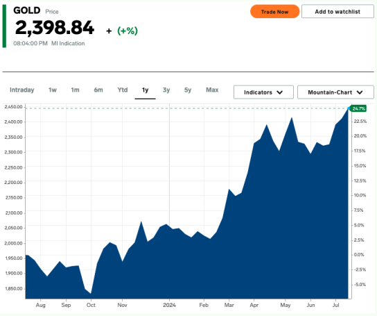		Compare this to say the October futures delivery price of $2,427.2.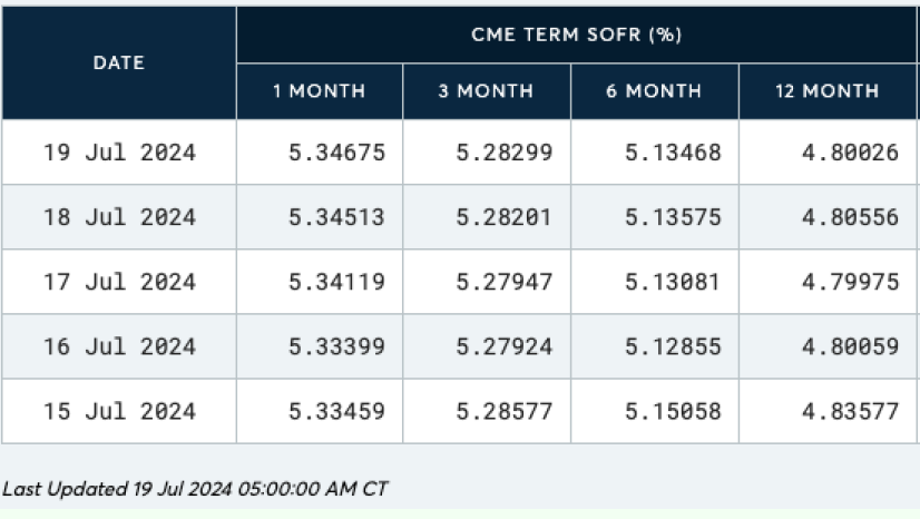

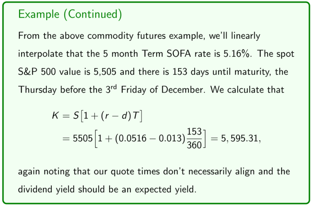
Equity contract pricing

In the case of share and index futures, we have an interest rate $r$ and a dividend yield of $q$. Hence the spot-forward parity relations become

$$K = S[1 + (r − q)T]$$

or

$$K = S(1 + r − q)^{T}$$

or

$$K = Se^{(r−q)T}$$

• going to use simple interest one because most of the interest rates given are simple
• No storage related costs in this case

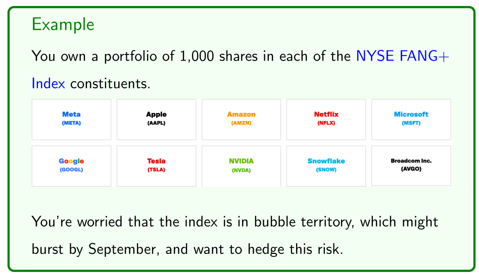
Example

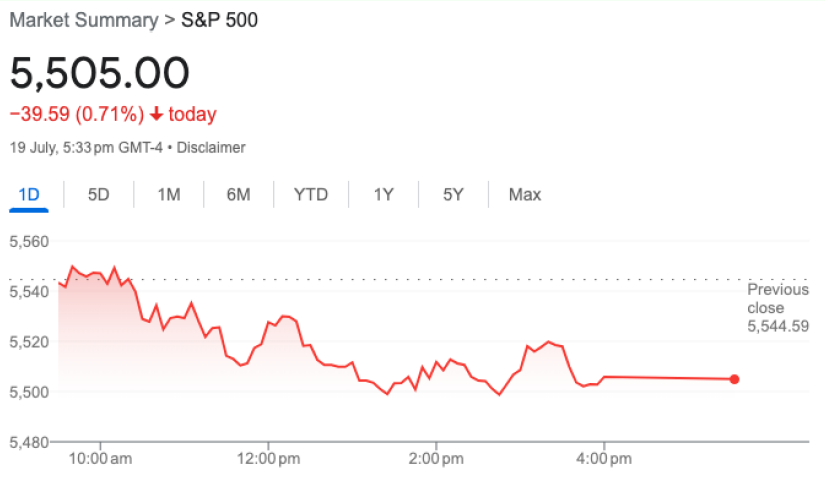
Futures Contract	Dividend Yields, average	Spot Price
Consider the December CME E-mini S&P500 futures contract.	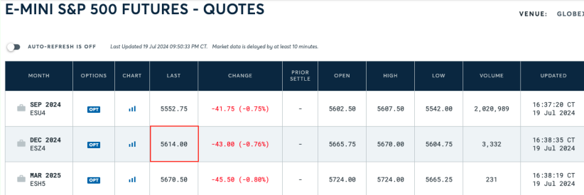The dividend yield of the S&P500 index is say 1.3%, and we’ll assume it’s an annual simple interest rate: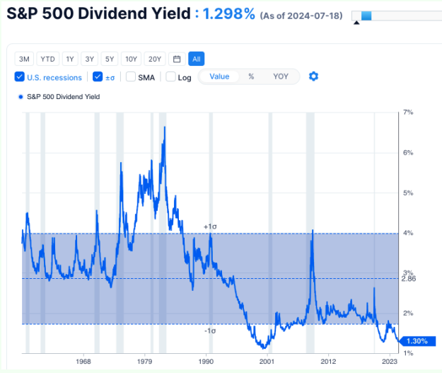

FX contract pricing

Spot-forward parity for FX contracts is best derived separately. The main complications are that we have to consider the interest rates in each country and we have to be careful about exchange rate quoting.

• Let $r_{d}$ be domestic interest rate and
• $r_{f}$ be the foreign rate.
• Let $S_{d:f}$ be the domestic:foreign spot exchange rate.
  • 1 unit of the domestic currency exchanges spot for $S_{d:f}$ units of the foreign currency.
• Let $K_{d:f}$ be the domestic:foreign forward exchange rate.

• currency contracts - instead of using cost of carry, best to derive the currency forward price/forward exchange rate separately

Two ways of earning interest over a time period T, namely:

1. Invest domestically at $r_{d}$ to get $1 + r_{d}T$ per unit invested.
2. Invest internationally:

• Buy $S_{d:f}$ units of foreign currency spot and simultaneously lock in the futures exchange rate of $K_{f:d}$ at time $T$.
• Invest $S_{d:f}$ at $r_{f}$ to get $S_{d:f} (1 + r_{f}T)$.
• Exchange this amount back into the domestic currency via the futures contract to end up with $S_{d:f} (1 + r_{f}T) K_{f:d}$

Both avenues must have the same final value or else there’s an arbitrage opportunity: Invest in the best avenue fund it with a reverse transaction (borrowing) in the other avenue.

• carry trade, exchange domestic currency
• investing domestically has to equal investing internationally through the carry trade

Hence, the no arbitrage relation is $1 + r_{d}T = S_{d:f} (1 + r_{f}T) K_{f:d}$ which we rearrange to get the covered interest rate parity relation

$$K_{f:d} = S_{f:d}\frac{1+r_{d}T}{1+r_{f}T}$$

Note that in the above we used $1/S_{d:f} = S_{f:d}$. Under compound interest:

$$K_{f:d} = S_{f:d}\left( \frac{1+r_{d}T}{1+r_{f}T} \right)^{T} \: \: \text{or} \: \: \: \: K_{f:d}=S_{f:d}e^{(r_{d}-r_{f})T}$$

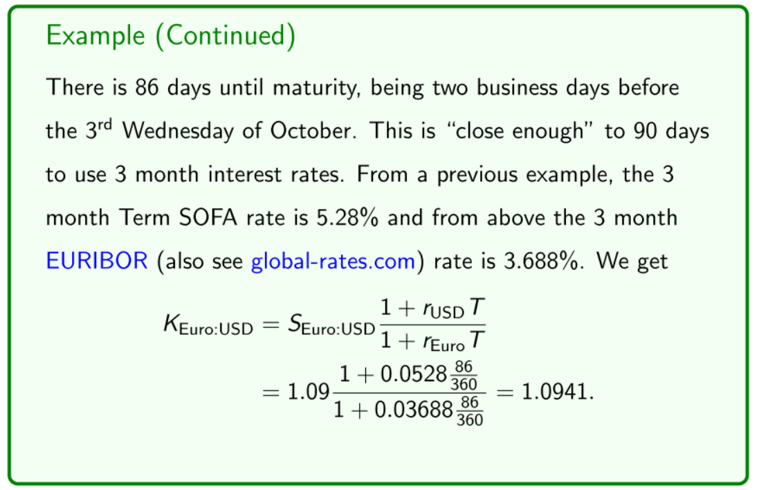
Example

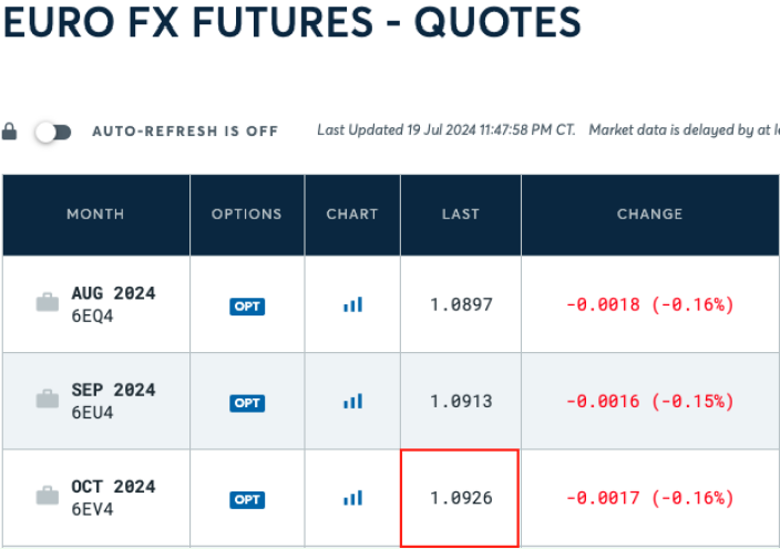
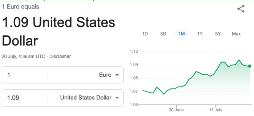
Let’s price the October CME Group Euro FX futures, which are futures contracts between the Euro and USD, the two most actively traded currencies in the world.

• Quote is $K_{Euro:USD}$.

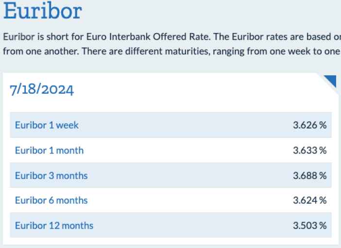
Contract Info	Current forwards	Spot	EURIBOR (Euro interest rate proxy)
Let’s price the October CME Group Euro FX futures, which are futures contracts between the Euro and USD, the two most actively traded currencies in the world. Quote is 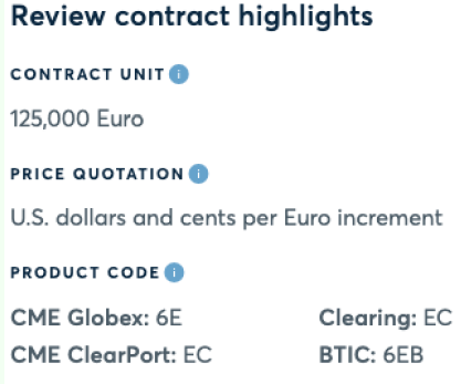$K_{text{Euro:USD}}$

• US dollar is the local currency
• how many units of the DC purchase one unit of the FC
• contract size is $125,000
• yield curve here 1 week, month, 3 months, 12 months

FRA Pricing

Recall that a $T_{1} \times T_{2}$ FRA is an OTC agreement to lock in a future borrowing or lending fixed rate $k$ starting at time $T_{1}$ , and finishing at time $T_{2}$ over a notional principal or face value F.

• Time $T_{1}$ is the FRA’s maturity date.
• The length of the time period is given by $T = T_2 − T_1$ .
• The fixed rate receiver hypothetically agrees to invest $F$ at time $T_{1}$ and receive the cashflow $F(1 + kT)$ at time $T_{2}$ .
• The fixed rate payer hypothetically agrees to borrow F at time $T_{1}$ and pay off the loan amount of $F(1 + kT)$ at time $T_{2}$.
• FRA are cash settled at maturity, time $T_{1}$.
• FRA are written over reference rates such as SOFR or EURIBOR.

Also recall that the payoffs at maturity to each party are given by

Fixed rate receiver payoff

$$= \frac{F(k-r)T}{1+rT}$$

Fixed rate payer payoff

$$= \frac{F(r-k)T}{1+rT}$$

where $r$ is the spot rate at maturity over the period $[T_{1}, T_{2}]$ of length T.

• We derived these payoff equations last week.

This week we want to price an FRA, which involves calculating the theoretically correct fixed rate k.

• positive for receiver, is the fixed rate $k$ is higher than the spot rate of the market $r$
  • vice versa for a payer, positive payoff is they 'lock in' a lower fixed rate $k$

The key insight is that the fixed rate $k$ is set so that the time $t = 0$ value of a FRA is $0$ to both the fixed rate receiver and payer.

So we want to calculate the time $t = 0$ values of a FRA to both parties:

• The fixed rate receiver of a $T_{1} \times T_{2}$ FRA hypothetically agrees to pay $F$ at time $T_1$ and receive $F(1 + kT)$ at time $T_2$.
• These cashflows are risk free so their present value is

$$V = -\frac{F}{1+r_{1}T_{1}} + \frac{F(1+kT)}{1+r_{2}T_{2}}$$

where $r_{1}$ and $r_{2}$ are the time $t = 0$ spot reference rates for the period from time $t = 0$ to times $T_{1}$ and $T_{2}$ , respectively.

• start at $t=0$

The value to the fixed rate payer is simply the negative of this.

• In either case, we find k by setting V = 0 and hence solving

$$\frac{F}{1+r_1T_1} = \frac{F(1+kT)}{1+r_2T_2}$$

Rearranging to:

$$1+r_2T_2 = (1+r_1T_1)(1+kT)$$

Hence, since $k$ is an interest rate starting at time $T_1$ and ending at time $T_2$ , it must be given by $k = r_{1,2}$, the implied forward rate over the time period $[T_{1}, T_{2}]$ embedded in the reference rate’s yield curve.

Rearrange the above to get:

$$k=\left( \frac{1+r_2T_2}{1+r_1T_1} -1 \right) \frac{1}{T}$$

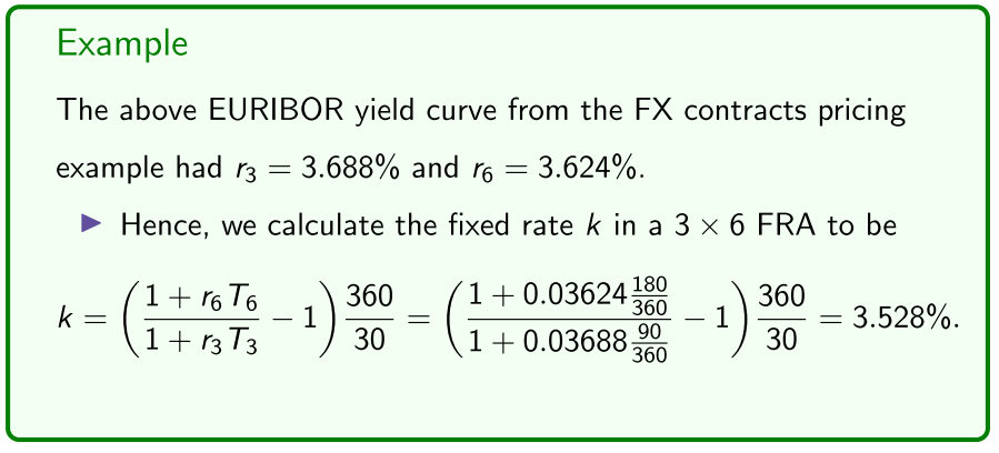
• should be 90 not 30 in the denominator

• starts from t=0 to t=2

• covers the time period now to the end of the contract
• total expression

Two ways to get a dollar invested

• invest at interest rate at that period OR
• invest at the interest rate you can lock in spot, up to the maturity date
• invest at the fixed rate you agree to at the FRA

Optimal Hedging

Last week we presented “perfect” hedging scenarios in which the:

• Underlying asset of a futures/forward contract is precisely the asset we want to hedge an exposure to,
• Number of assets we held was divisible by the contract multiplier m, enabling us to use an integer number of contracts.
• Contract maturity date is precisely our desired hedging date.

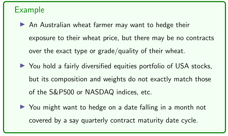
Perfect hedging scenarios are rare in practice:

So far presented unrealistic hedging

• Large diversified share portfolio, there is no futures contract that can perfectly hedge
• not exactly over the asset that we hold
• contract multiplier might not be divisible
• date might not be the exact maturity date
• Use some sort of futures contract
  • not sure if contract will materialise on maturity date

Example

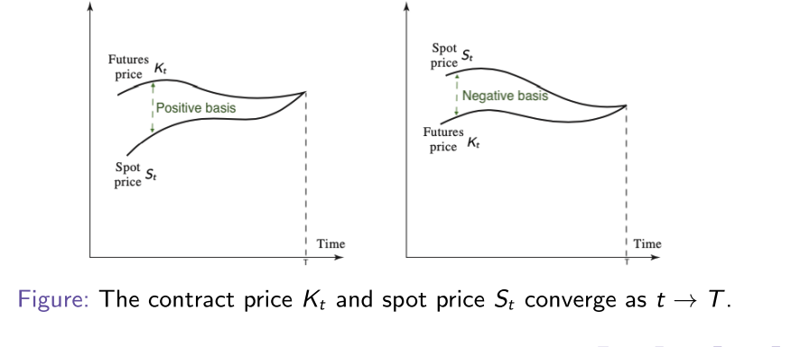
Basis Risk

We saw above that the contract price $K$ is usually different to the spot price S of the underlying asset. Our pricing equations, such as

$$K=Se^{(r+s-q)T}$$

for commodity futures, tell us that the difference between $K$ and $S$, which we call the basis, is due to the cost of carry $r + s − q$.

• As the cost of carry changes over time, the basis changes, introducing basis risk: $K$ may not be perfectly correlated with $S$.

Remark The situation is even more complicated if the asset we hold and want to hedge is not the same as the contract’s underlying asset.

• interest rates, storage costs change every day
• difference between contract price and spot price
  • when we do perfect hedging

The time $t$ basis $B_t$ is the difference between $K_t$ and $S_t$, namely:

$$B_{t} = K_{t}-S_{t}$$

Note that the basis approaches 0 over time, and $K_{T}=S_{T}$ at maturity.

hedging with a different maturity date, don't know what the basis is going to be

• basis risk

Optimal hedging

Optimal hedging basically means minimising basis risk. Suppose:

• We hold $Q$ units in an asset at time $t = 0$.
  • Its price at time $t$ is denoted by $A_{T}$.
• We want to sell our holding at time $t$.
  • We want to hedge our exposure to a fall in the asset price.
• There is a futures contract maturing at time $T$, with $t < T$.
  • The underlying asset of the futures contract $S$ may not necessarily be the same as the asset $A$ we hold.
• We short $h$ units of the futures contract at time $t = 0$ for $K$.
• We sell our asset holding and close out the futures position at time $t$.

How many contracts $h$ should we short?

• minimise basis risk
• Hypothetical time t=0
• exposed to the price of the asset falling
  • asset to short to hedge this risk
  • may not necessarily be on the same date
• We still sell the contract, even if they might not be exactly the same (but are correlated)
  • probably use the contract to hedge exposure
  • given all uncertainties (basis risk)

Optimal hedging

At time $t$, the liquidation value (net cashflow) of our position is

$$L_{t}=QA_{t}+h(K-K_{t})m$$

• $Q$ is the number of units we hold in our asset.
• $A_t$ is the time $t$ price of our asset (we let $A = A_0$ ).
• $h$ is the number of futures contracts we shorted.
• $K$ is the contract price at time $t = 0$ when we went short.
• $K_t$ is the contract price at time $t$ when we went long to close out.
• $m$ is the futures contract multiplier.

• sell our asset holding at $t$

We were holding Q units, and going to sell at $A_{t}$

• total amount from liquidating everything, closing out our holdings
• $QA_{t}$ when we sell our asset
• $h(K-K{t})m$ when we liquidate our hedged position

In perfect hedging, lock in perfect liquidation value

• Liquidation value is certain
• Asset we hold is the asset in the contract
• $t=0$ when we establish our hedge, dont know our asset price at $t$
• minimise the variance/volatility on the liquidation day

Perfect hedging, lock in liquidation value

• optimal - minimise risk/volatility
• Get as much certainty as possible in liquidation value

In an imperfect hedging scenario, in which there is basis risk, we choose $h$ that minimises the variance in the liquidation value $L_{t}$.

Then $h$ is called the minimum variance or optimal hedge quantity.

• At time $t = 0$, $A_{t}$ and $K_{t}$ are unknown, thus random variables.

We use the following notation:

• $σ_{A_t}$ is the standard deviation (volatility) in $A_t − A$.
• $σ_{K_t}$ is the standard deviation (volatility) in $K_t − K$.
• $ρ$ is the correlation between $A_t − A$ and $K_t − K$.

$A_{t}$ and $K_{t}$ are unknown and not necessarily correlated

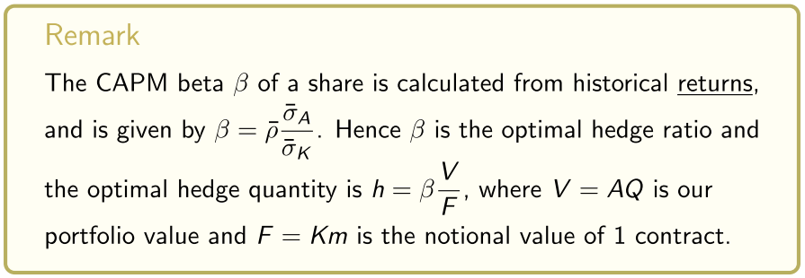
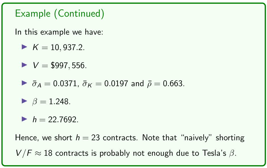
We can prove that the optimal or minimum variance hedge quantity $h$, which minimises the variance in the above liquidation value, or equivalently minimises basis risk, is given by

$$h=\rho \frac{\sigma_{A_{t}}Q}{\sigma _{K{t}}m}$$

Remark The number

$$\frac{\sigma_{A_{t}}Q}{\sigma _{K{t}}m}$$

is called the minimum variance or optimal hedge ratio.

• proportion of futures contracts to 1 futures contract
• Can calculate them with historical data

The optimal hedge quantity is then given by

$$h = \bar{\rho} \frac{\bar{\sigma}_{A}Q }{\bar{\sigma}_Km}$$

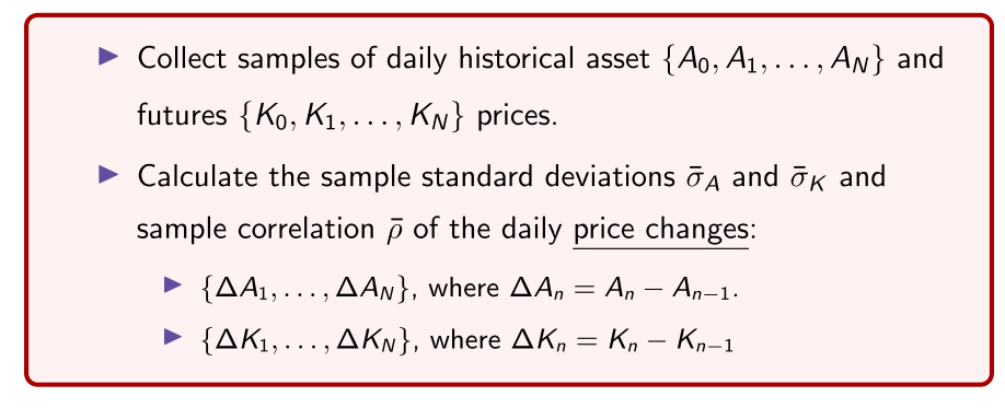
Also, suppose that in the above we used daily returns $(A_n − A_{n−1} )/A_{n−1}$ and $(K_n − K_{n−1})/K_{n−1}$ to calculate $\bar{\sigma}_{A}$, $\bar{\sigma}_K$ and $\bar{\rho}$.

• two sample data sets of price increments
• calculate the variance, and the correlation between the two
• optimal hedge quantity given by the expression

• Then the optimal hedge quantity is given by

$$h = \bar{\rho} \frac{\bar{\sigma}_{A}V }{\bar{\sigma}_KF}$$

Where

$$V = AQ \; \; \; \text{and} \;\;\;\; F=Km$$

• optimal standard deviation of standard returns of contract price

• Sample correlation of daily returns

• Still the hedge ratio, multiplied by the asset value of the face value of the asset

• V could represent a portfolio value

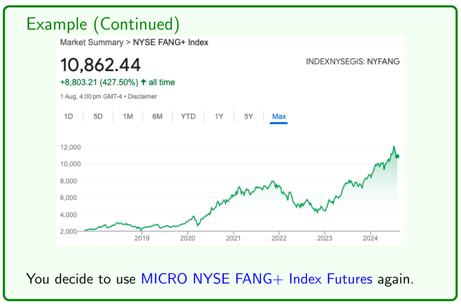
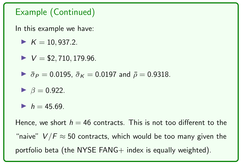
Example

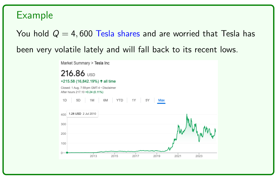
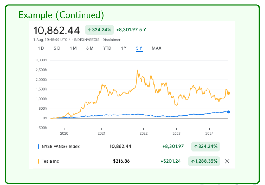
Example 2

We now calculate the optimal hedge quantity of a portfolio of shares.