Lecture 4

• Plain vanilla options - basic kinds of options
  • there are more exotic options, complicated derivative securities also

Introduction to options

Recall that there is two types of plain vanilla European options:

• Call option: Gives the holder the right but not the obligation to buy the underlying asset for the strike price $K$ on the expiry date $T$.
• Put option: Gives the holder the right but not the obligation to sell the underlying asset for the strike price $K$ on the expiry date $T$.

Also recall that an American option gives the holder these rights at any point in time up to and including the expiry date $T$.

• also called strike price, or exercise price, or $k$
• option premium or value, or price.
• For options we call it options date (or maturity date)

The option writer is “at the mercy of” the buyer.

• We say that an option has asymmetric rights.

• Assume no counterparty risk - we assume they are going to do it

Notation

• We work on a given time interval $0 ≤ t ≤ T$ where:
  • Time $t = 0$ is the date we enter into a contract.
  • Time $T$ is the expiry date.
  • Time $t$ is some intermediate date $0 ≤ t ≤ T$.
• $S_t$ is the underlying asset’s price at time $t$.
  • We write $S = S_{0}$ to reduce notation.
• $r$ is the risk free rate.
• $K$ is the strike or exercise price (some authors use X).
• $C_{t}$ and $P_{t}$ are the call and put prices (premiums) at time $t$.
  • Again, we write $C = C_{0}$ and $P = P_{0}$.

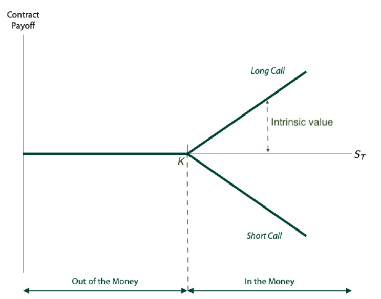
Asymmetric rights: The holder (long position) has payoffs at expiry of

• call holder payoff = $\max \{ 0, S_{T} − K \}$
• put holder payoff = $\max \{ 0, K − S_{T} \}$

and the writer’s (short position) payoffs are the negative of these:

• call writer payoff= $− \max \{ 0, S_{T} − K \}$,
• put writer payoff= $− \max \{ 0, K − S_{T} \}$.

thinking about payoffs only

• Beauty of options for holders is never non-negative
• not going to incur a loss besides the premium they pay

Option Payoffs and profits

Call options	Put options

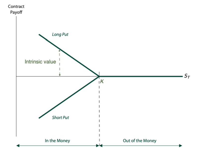Options intrinsic value

At any time t, an option’s intrinsic or exercise value (IV) is

call $IV_{t} = \max \{ 0, S_{t} − K \}$

and put $IV_{t} = \max \{ 0, K − S_{t} \}$

(payoff if the option expired at time t).

At time $t$ an option is:

• In the money if it has positive intrinsic value:
  • $K < S_{t}$ for a call option.
  • $S_{t} < K$ for a put option.
• At the money if $S_{t} = K$ (intrinsic value is 0).
• Out of the money if its intrinsic value is 0 and $S_{t} \ne K$
  • $S_{t} < K$ for a call option.
  • $K < S_{t}$ for a put option.

• in the money, positive payoff

The above motivates using the idea of no arbitrage to justify the taker having to pay the option price or premium to the writer:

• The holder’s payoff at expiry is nonnegative (positive or zero).
• If options required no upfront premium, then by definition this would be an arbitrage opportunity for the holder:
  • No upfront cashflow.
  • No risk of loss.
  • Chance of a positive payoff.

Remark Developing complex mathematical models that calculate the fair value of an option’s premium takes up a lot of space in the world of quant finance in both industry and academia.

• Have a positive value at any point in time
• Option holder, payoff is not negative you can never lose
  • If the option costs nothing, you would enter into more and more
  • Would be an arbitrage situation and would not hold Premium takes up a

To calculate trading profits, the above payoff s need to be modified to incorporate the premium paid/received. The option taker’s profits are:

• call holder profit = $\max \{ 0, S_T − K \} − C$,
• put holder profit = $\max \{ 0, K − S_T \} − P$

and the writer’s (short position) profits are the negative of these:

• call writer profit = $C − \max \{ 0, S_T − K \}$,
• put writer profit = $P − \max \{ 0, K − S_T \}$.

• profits, profit diagram
• same as payoff diagram and including the premium

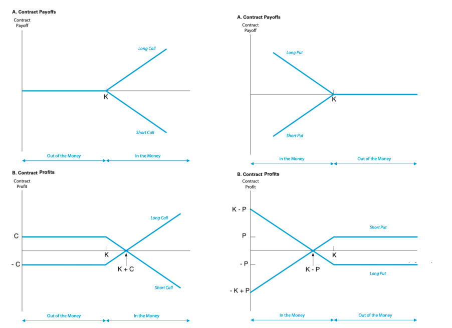
So the premium gives the writer a chance of a profit, but exposes them to the risk of significant loss, unlimited in the case of call options:

• Calls and puts:
  • Holder: Loss is limited to the premium paid $C$ or $P$.
  • Writer: Profit is limited to the premium received $C$ or $P$.
• Call options:
  • Holder: Profit is unlimited and equal to $S_{T} − K − C$ for $S_{T} > K$.
  • Writer: Loss is unlimited and equal to $S_{T} − K − C$ for $S_{T} > K$.
• Put options:
  • Holder: Profit is potentially large and as much as $K − P$ for $S_{T} = 0$.
  • Writer: Loss is potentially large and as much as $K − P$ for $S_{T} = 0$.

Exchanges have margin mechanisms for short options positions.

Options vs futures/forwards

Fundamental differences between futures/forwards and options:

• Obligations:
  • Futures/forwards: Both parties must transact.
  • Options: The taker/holder gets to choose.
• Payoffs:
  • Futures/forwards: Symmetric.
  • Options: Asymmetric (favour the taker/holder).
• The “price” or value:
  • Futures/forwards: The actual contract price $K_{t}$.
  • Options: The premium $C_t or P_{t}$ (the strike price K is fixed).
• Upfront cashflow:
  • Futures/forwards: $K_{t}$ is set so they have 0 upfront value/cashflow.
  • Options: The taker pays premium $C_{t}$ or $P_{t}$ upfront to the writer.

• Price of a futures or forwards, the actual price of the contract ($k$)
• In contracts it is the price of the premium

Options markets

We look at the main exchange traded options markets and contracts for:

• Equities:
  • Individual share and ETFs.
  • Share index.
• Currencies.

While doing this we don’t present basic speculation and hedging examples since these we devote a whole lecture to this in a few weeks time. We also cover interest rate derivatives later in the course.

Commodity options

Note also that commodity options are not as actively traded as commodity futures so we’ll skip looking at commodity options:

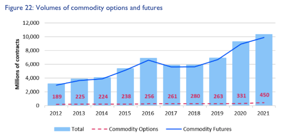
Nowhere near as popular

Equity Options

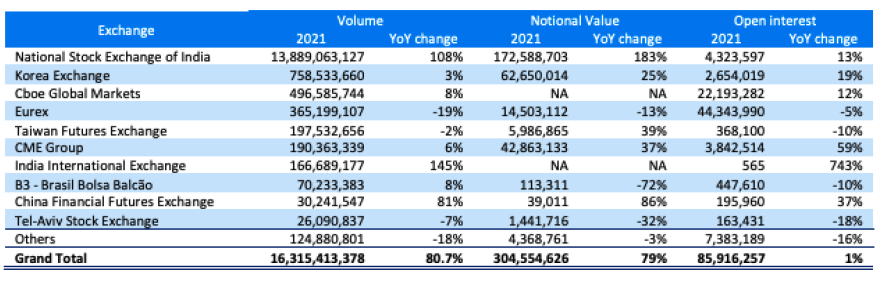
Equity options are very popular and heavily traded products. Below gives volumes for all exchange traded derivatives (options and futures).

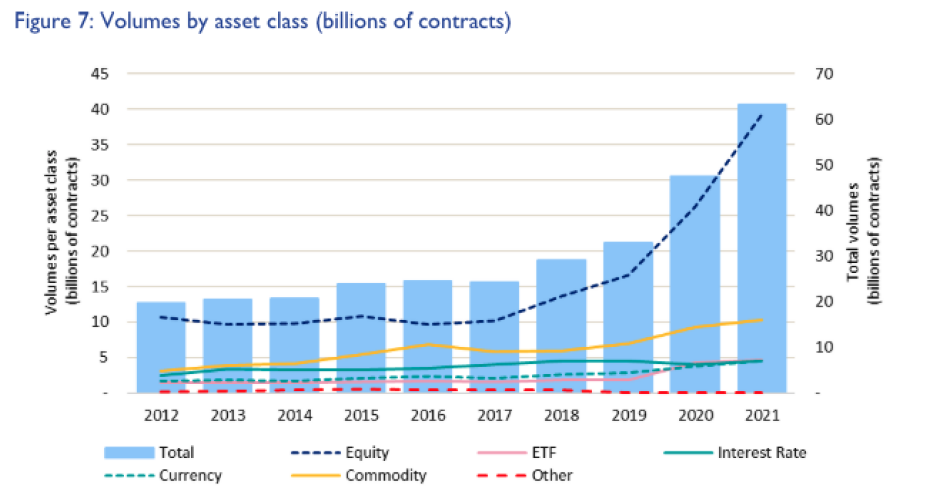
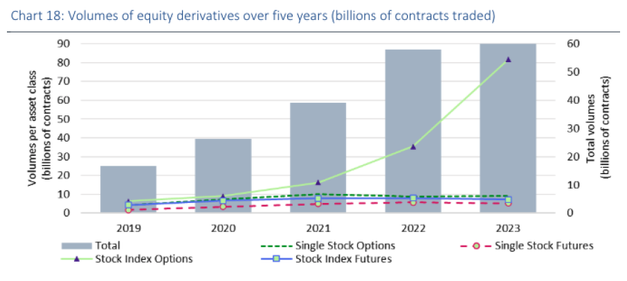
And out of the very large volume of equity derivatives trading worldwide from the previous slide, it’s mostly equity options trading:

Share and ETF options

Starting with individual share and ETF options, most trading by volume is in the USA (NASDAQ, CBOE, NYSE, MIAX, ISX combined).

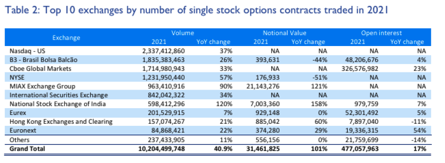
And the heaviest share options trading is in Apple and Tesla:

Contracts and product specifications

• Symbol,
• Underlying asset (normally 100 shares) $m=100$
• Strike prices go up in discrete increments
  • A lot of options contracts (maturing 1 month, 3 months, etc)
  • At the money stock prices are usually listed first
• Expiration date
• Expiration month
• Expiry dates available on the exchange
• Most share options are American
  • Also offer European individual share options
  • Short party can only earn the premium
  • Go short an option, loss if potentially quite huge, will have a daily margin mechanism

Options on ASX

• American and European
• Exercise style
• Exercise price
  • If your option is physically in the money, may have to provide the shares (long/put) have to physically provide the shares

Individual share options

• typically American

Index options

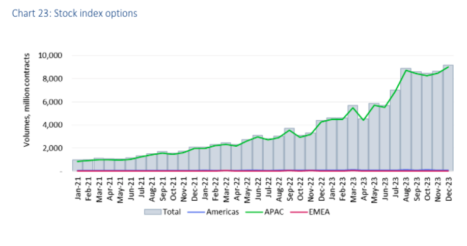
Turning to index options, it has taken off worldwide:

• bunch of retail everyday investor trading small amounts
• American is bigger in terms of the size of the contract

Share index contract specifications

• Contract type, European,
• CBOE S&P500 Index options:
  • American contracts, very common
• Cash settled, not physically settled

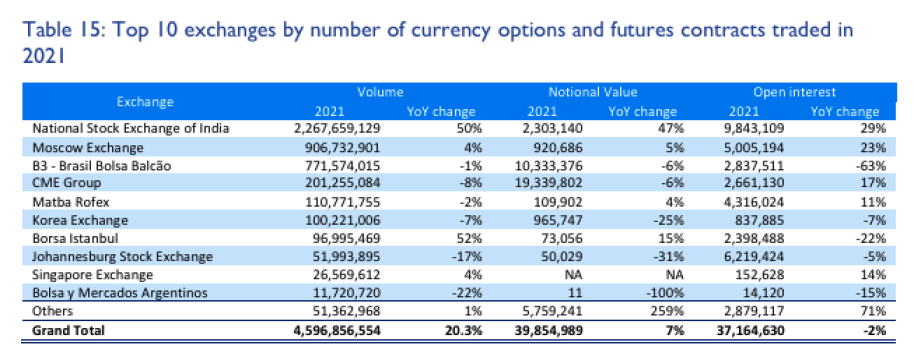
Currency Options

Turning to currency options, they previously didn’t but now do have roughly the same trading volume as currency futures:

• always cash settled

ASSIGNMENT

• what contracts were available to him, payoffs available, etc.

Pricing relationships and Bounds

That’s enough for looking at the major exchange traded options contracts worldwide. Note that, as we also know, OTC markets are huge and options contracts traded on them tend to be less standardised, with more complex and exotic options being traded. We cover some of these exotic options later in the course.

• We now turn to option pricing bounds and put-call parity.

Put-call Parity

Developing mathematical models for pricing options (calculating the fair value of the option premium), such as the Black-Scholes option pricing model, is a major part of the theory and practice of options.

• We cover the basics in later lecture notes, starting next week with the celebrated Black-Scholes option pricing model.
  • But before covering formal option pricing models, we can use no arbitrage arguments to show that there are pricing relations and bounds that at least plain vanilla options prices must adhere to and satisfy.
• We start with the (possibly already familiar) put-call parity relation.

• Basic arbitrage arguments
  • certain relationships that need to hold
  • options premiums at need to hold
• Use certain pricing bounds to guide where you are going

Put-call parity gives a strict relation that must hold, due to no arbitrage arguments, between the prices P and C of European put and call options over the same underlying asset and with the same strike K and expiry T:

Form a portfolio long 1 European call and short 1 European put, both with the same underlying, strike and expiry.

This portfolio’s current price is C − P and its payoff at expiry is

$$\text{portfolio payoff} = \underbrace{\max\{0, S_T - K\}}_{\text{long call}} - \underbrace{\max\{0, K - S_T\}}_{\text{short put}}$$

$$= S_T - K$$

This is easy to show:

• If $S_{T} > K$ then the payoff is $S_{T} − K − 0 = S_{T} − K$.
• If $S_{T} < K$ then the payoff is $0 − (K − S_{T} ) = S_{T} − K$.
• Finally, if $S_{T} = K$ then the payoff is $0 − 0 = 0 = S_{T} − K$.

But $S_{T} −K$ is precisely the payoff of a long futures contract position over the underlying with contract price K and maturity date $T$.

So the value $C − P$ of this portfolio long 1 call and short 1 put must equal the value of a long futures position with price $K$.

• Since their payoff s are equal, or else there is an arbitrage opportunity.

• Let $X=Se^{rT}$ be the theoretically correct futures contract price.

• If we’re long at K we could go short to close out the position at X.

• The value of this long futures contract position is

$$V^{\text{long}}=e^{-rT}(X-K)$$

So put-call parity is $C − P = e^{−rT}(X − K)$, which we rearrange to

$$C − P = S − e^{−rT}K$$

noting that $e^{−rT} X = e^{−rT} Se^{rT} = S$.

• Theoretically exit out of the contract $X$ Put call parity
• price of a long call and a short put option must equal the value of a long futures contract

Remark Put-call parity is also useful for equity options, in which we assume a continuously compounded annual dividend yield $q$.

• Here, the theoretically correct futures price is $X = Se^{(r−q)T}$ so put-call parity

$$C − P = e −rT (X − K)$$

becomes

$$C − P = e^{−qT}S − e^{−rT}K$$

Note also that we tend to use continuous compounding for options.

Option pricing bounds

We now present pricing bounds that option prices must adhere to.

• If they don’t satisfy these bounds then arbitrage opportunities exist.

First note that American options are worth at least as much as European options over the same underlying asset and with the same strike and expiry:

$$0 ≤ C_{Eu} ≤ C_{Am}$$

and

$$0 ≤ P_{Eu} ≤ P_{Am}$$

because American options can be exercised any time up to and including expiry, but European options can only be exercised at expiry.

• American options provide more flexibility and opportunity to profit.

• over the same underlying asset, same strike price, etc.

And American options are worth at least their intrinsic (exercise) value:

$$\max{0, S − K} ≤ C_{Am}$$

and

$$\max{0, K − S} ≤ P_{Am}$$

(lower pricing bounds) because they can be exercised immediately

• At any point in time you can exercise and realise that in an American Options
  • At least as much as the actual payoff

Also, American calls can never be worth more than the underlying spot price, and American puts can never be worth more than the strike:

$$C_{Am} ≤ S$$

and

$$P_{Am} ≤ K$$

(upper pricing bounds). Proving this is left as a tutorial exercise.

Combining the lower and upper bounds from the previous two slides leads to the important pricing bounds for American options:

$$\max \{ 0, S − K \} ≤ C^{Am} ≤ S \: \: \text{and} \: \: \max \{ 0, K − S \} ≤ P^{Am} ≤ K$$

European options

Turning to European options, we can tighten an upper bound for puts to

$$0 \le P^{Eu} \le Ke^{-rT}$$

because a European put can only be exercised at expiry, where it is known with certainty that their maximum payoff at expiry is $K$.

Remark From this, deep in-the-money European puts can have negative time value (their premium can be less than their intrinsic value).

• Their maximum payoff is $K$. So if they’re already deep in the money, not much more payoff can be realised at expiry, but the underlying asset could still move unfavourably.

• If you hold a European put option deep in the money (price of the asset is really low)
  • European option, have to wait to expiry, could ruin payoff

Options trader, deep in the money very likely it gets exercised

• Trade options and short, have to be careful in situations where people exercise

Writing a naked option - writing an option with no asset

• opposite to being totally covered

Furthermore, we can use put-call parity

$$C^{Eu} - P^{Eu} = e^{-qT}S-e^{-rT}K$$

to derive further lower bounds on European options.

• Since option prices are nonnegative, for European calls we get

$$\max \{ 0, e^{-qT}S-e^{-rT}K \} \le C^{Eu} \le S$$

• have upper pricing bounds, $\le$ the stock price
• Lower pricing bound, if we remove $-P^{Eu}$ which must have a positive premium, then removing it from the above equation would mean $e^{-qT}S-e^{-rT}K$ must be less than $C^{Eu}$

and for European puts we get

$$\max(0, e^{-rT}K - e^{-qT}S) \le P^{Eu} \le Ke^{-rT}$$

• similar reasoning to above.

No dividends: No early exercise of American calls

We actually have everything needed to show that early exercise is never optimal for an American call option on a non-dividend-paying stock:

• Under no dividends, so $q = 0$, from above we start with

$$\max (0, S − e^{−rT}K) ≤ C^{Eu} ≤ C^{Am}$$

• If $r > 0$ then $e^{−rT} K < K$ and we get a strict inequality

$$\max(0, S − K) < \max (0, S − e^{−rT}K) ≤ C^{-rT} ≤ C^{Am}$$

But $\max(0, S − K)$ is just the call’s intrinsic value. So if there’s no dividends, call options will always have strictly positive time value.

• no value in early exercising a call option on a non-dividend option paying stock
• Actual price of an American option
• worth exercising if the theoretical price equals its intrinsic value
  • always be valued greater than the payoff

• Under no dividends you never exercise an American call early.
  • The early exercise feature of American calls is worthless.
• So the American and European call prices are equal: $C^{v} = C^{Am}$.
• And the pricing bounds for European and American calls combine:

$$\max(0, S-e^{-rT}K) \le C^{Eu} \le S$$

• option of a non-dividend paying asset, lower bound is the same

Remark If there is dividends, it may be optimal to exercise an American call on the day before the ex-dividend date. In any case early exercise may be optimal for deep in the money American puts.

Summary of pricing bounds

$$\max (0, S − K) ≤ C^{Am} ≤ S$$

$$\max (0, K − S) ≤ P^{Am} ≤ K$$

European:

$$\max(0, e^{-qT}S-e^{-rT}K) \le C^{Eu} \le S$$

$$\max(0, e^{-rT}K - e^{-qT}S) \le P^{Eu} \le Ke^{-rT}$$

Call options on non-dividend paying underlying:

$$\max(0, S - e^{-rT}K) \le C^{Eu} = C^{Am} \le S$$

Time value

• And what exactly is time value?

From above, we noticed that call options on non-dividend-paying stocks have a premium that is strictly larger than the option’s intrinsic value.

• We define an option’s time value as the difference between the option premium and its intrinsic value:

$$\text{time value = premium − intrinsic value}$$

A better way to think of it is that the option’s premium is made up of the option’s intrinsic value plus the option’s time value:

$$\text{premium = intrinsic value + time value}$$

• options are worth more than their intrinsic value
  • fair bit of time to expiry
  • can still move in a direction that favours you
  • can move in opposite direction, but loss is capped

• Intrinsic value: Represents the option’s payoff if the option expired at that moment in time - the exercise value.
• Time value: Represents the possibility that the price of an option’s underlying will move favourably for the option holder before expiry.

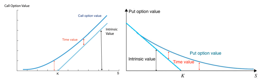
• value of the premium of the call option is a small curve
• positive time value
• given a fixed strike price

European put option deep in the money, can have a negative time value