Lecture 5

The Black-Scholes European option pricing model is a mathematical equation for pricing plain vanilla European call and put options.

In general the “Black-Scholes model” is a mathematical framework in which we derive mathematical models for pricing derivatives.

In the Black-Scholes framework, some types of derivatives have nice equations for their price or value, but most do not. When they don’t, we have to use numerical methods to approximate the solution, such as:

• Lattice based method like the binomial and trinomial models.
• Monte Carlo simulation methods.
• Numerically solving partial diff erential equations.

• Focus on the black-Scholes framework
  • Standard market model
  • Can derive a clean neat price for the derivatives
  • Not going to focus on complex derivative securities
• Model itself is pretty unique, and do have a formula for their price
  • most models you cannot derive a formula, sometimes they don't even exist
• Use numerical techniques
  • Not going to solve partial differential equations
    • which represents the price of the derivative

This week we cover the Black-Scholes option pricing model for:

• The basic equations for European options.
• European options on equities or indices that pay a dividend yield $q$.
• European currency options, being mindful of the domestic $r_{d}$ and foreign $r_{f}$ risk-free rates, as well as currency quoting conventions. In later weeks we cover numerical methods for other types of options that don’t have neat Black-Scholes pricing equations.

• numerical methods will be in-semester test

Quite simply, the Black-Scholes European call option pricing model is

$$C = S\mathcal{N} (d_{1}) − Ke^{−rT}\mathcal{N} (d_{2})$$

Where:

$$d_{1} = \frac{\log \frac{S}{K} + (r+\frac{1}{2}\sigma ^{2})T}{\sigma \sqrt{T}}$$

And

$$d_{2} = d_{1} - \sigma \sqrt{T}$$

$$= \frac{\log \frac{S}{K} + (r -\frac{1}{2}\sigma ^{2})T}{\sigma \sqrt{T}}$$

Let’s recall the notation and variables in the Black-Scholes model:

Notation and variables

• The current date is time $t = 0$.
• $C$ is the current European call option premium.
• $T$ is the expiry date (and also time to expiry).
• $S$ is the current price of the underlying asset.
• $r$ is the risk-free rate.
• $K$ is the exercise or strike price.

First, $\sigma$ is the volatility of the underlying asset, which we can take as the standard deviation of its continuously compounded annual returns.

• $\sigma$ can be calculated from historical data as follows:

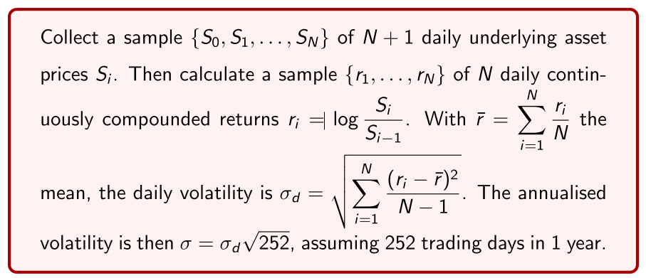
• sample of daily prices of the asset
• N+1 price observations, N daily returns
• Calculate the sample standard deviation

Traders don't use historical data, they use market

Second, $\mathcal{N}(x)$ is the CDF evaluated at $x$ of a standard normal random variable $X$. It gives the probability that $X$ is less than or equal to $x$:

$$\mathcal{n}(X) = \mathbb{P}(X \le x) = \frac{1}{\sqrt{2 \pi}} \int^{x}_{- \infty } e^{- \frac{z^{2}}{2}} dz$$

Graphically, it’s the area under the standard normal PDF:

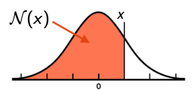
• Probability standard normal random variable $\le$ x
• Area under the curve of standard probability density function
• Use computers to calculate it for us

Example in code

Python

In [1]: from scipy . stats import norm
In [2]: x = 0.75
In [3]: N = norm.cdf(x) # SciPy ’s norm.cdf () is N()
In [4]: N
Out [4]: 0.7733726476231317

Black Scholes Model

In R

S = 50
K = 50
r = 0.05
T = 1/2
sigma = 0.25
d1 = (log(S/K) + (r + 0.5* sigma ^2)*T)/( sigma *sqrt(T))
d2 = d1 - sigma *sqrt(T)
C = S* pnorm (d1) - K*exp(-r*T)* pnorm (d2)

Gives:

> C
[1] 4.130008

In Python

import numpy as np
from scipy . stats import norm
S = 50
K = 50
r = 0.05
T = 1/2
sigma = 0.25
d1 = (np.log(S/K) + (r + 0.5* sigma **2)*T)/( sigma *np.sqrt(T))
d2 = d1 - sigma *np.sqrt(T)
C = S*norm.cdf(d1) - K*np.exp(-r*T)*norm.cdf(d2)

gives

In [1]: C
Out [1]: 4.130007599671615

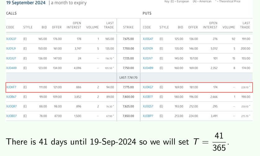
Use the yfinance Python module to calculate the historical volatility of the S&P/ASX 200 Index and price some September index option contracts, where here we’ll ignore dividends (for now).

Interest Rates	Option Prices

 import numpy as np , yfinance as yf
 from scipy . stats import norm
 P = yf. download ("^AXJO")["Adj Close "]
 ret = np.log(P).diff (1). dropna ()
 sigma = np.std(ret)*np.sqrt (252)
 K = 7775; S = 7761.7; T = 41/365
 r = (0.042923+0.04335) /2 # average of 1 & 2 month BBSW rate
 d1 = (np.log(S/K) + (r + 0.5* sigma **2)*T)/( sigma *np.sqrt(T))
 d2 = d1 - sigma *np.sqrt(T)
 C = S*norm.cdf(d1) - K*np.exp(-r*T)*norm.cdf(d2) # call price
 P = K*np.exp(-r*T)*norm.cdf(-d2) - S*norm.cdf(-d1) # put price

This code gives σ = 0.15375 and European call and put prices

1 In [1]: C
2 Out [1]: 171.73
3 In [2]: P
4 Out [2]: 147.45

• options prices potentially be off - using historical volatility and options traders don't do that
  • us their own market conventions

Black-Scholes Model Puts

$$P = Ke^{−rT}\mathcal{N} (-d_{2}) - S\mathcal{N} (-d_{1})$$

where all variables and notation are as above.

• Alternatively, we can use put-call parity:

$$P = C + e^{−rT}K − S$$

We check that they agree, using the original “generic” example above:

P = K*np.exp(-r*T)*norm.cdf(-d2) - S*norm.cdf(-d1)
P1 = C + np.exp(-r*T)*K - S # using put -call parity

• Exam situation, formula will be provided

Incorporating dividends

We now incorporate dividends into the Black-Scholes European option pricing equations, in order to more accurately price equity options.

Incorporating a continuously compounded dividend yield $q$ into the basic Black-Scholes model is relatively easy. We can show that the pricing equations for European call $C$ and put #$P$ options become

$$C = Se^{-qT}\mathcal{N} (d_{1}) − Ke^{−rT}\mathcal{N} (d_{2})$$

$$P = Ke^{−rT}\mathcal{N} (-d_{2}) - Se^{-qT}\mathcal{N} (-d_{1})$$

Where:

$$d_{1} = \frac{\log \frac{S}{K} + (r - q + \frac{1}{2}\sigma ^{2})T}{\sigma \sqrt{T}}$$

And

$$d_{2} = d_{1} - \sigma \sqrt{T}$$

$$d_{2} = \frac{\log \frac{S}{K} + (r - q - \frac{1}{2}\sigma ^{2})T}{\sigma \sqrt{T}}$$

• Black Scholes prices of plain vanilla options including dividends

Example

import numpy as np , yfinance as yf
from scipy . stats import norm
XJO=yf. download ("^AXJO")["Adj Close "]
ret=np.log(XJO).diff (1). dropna (). rename (" returns ")
sigma =np.std(ret)*np.sqrt (252)
K =7775; S =7761.7; T =41/365; q =0.042 # dividend yield 4.2%
r =(0.042923+0.04335) /2 # average of 1 & 2 month BBSW rate
d1 =( np.log(S/K)+(r-q +0.5* sigma **2)*T)/( sigma *np.sqrt(T))
d2=d1 - sigma *np.sqrt(T)
C=S*np.exp(-q*T)*norm.cdf(d1)-K*np.exp(-r*T)*norm.cdf(d2)
P=K*np.exp(-r*T)*norm.cdf(-d2)-S*np.exp(-q*T)*norm.cdf(-d1)

This code gives European call and put prices

In [1]: C
Out [1]: 152.87
In [2]: P
Out [2]: 165.12

Remark:

Some reasons for inaccurate S&P/ASX 200 Index option prices:

• We’re using historical volatility for σ but in practice options traders tend to use the Black-Scholes model with “rules of thumb” and their own estimates of σ.
• Our dividend yield may not be accurate: We assumed a continuously compounded yield. It should be a forecast. And should we incorporate dividend imputation/franking?
• The time stamps on our data don’t align.

Currency Options

When applying the Black-Scholes model to pricing currency options, we need to be mindful about the currency quoting conventions of $S$ and $K$, as well as the handling of the domestic $r_{d}$ and foreign $r_{f}$ interest rates.

• Let’s recall our currency quoting convention:

Let $S_{f:d}$ and $K_{f:d}$ be the spot and strike prices of 1 unit of the foreign currency (the underlying asset) in terms of the domestic currency.

The modification to the Black-Scholes model is relatively easy:

• It turns out that we view the foreign risk-free rate $r_f$ as the “dividend” on the underlying asset (the foreign currency):

• Cutting out messiness, European options on currencies is the same as dividend yields

$$C_{f:d} = S_{f:d}e^{-qT}\mathcal{N} (d_{1}) − K_{f:d}e^{−rT}\mathcal{N} (d_{2})$$

$$P_{f:d} = K_{f:d}e^{−rT}\mathcal{N} (-d_{2}) - S_{f:d} e^{-qT}\mathcal{N} (-d_{1})$$

Where:

$$d_{1} = \frac{\log \frac{S_{f:d}}{K_{f:d}} + (r - q + \frac{1}{2}\sigma ^{2})T}{\sigma \sqrt{T}}$$

and

$$d_{2} = d_{1} - \sigma \sqrt{T}$$

$$= \frac{\log \frac{S_{f:d}}{K_{f:d}} + (r - q - \frac{1}{2}\sigma ^{2})T}{\sigma \sqrt{T}}$$

This is sometimes called the Garman-Kohlhagen (GK) equations, who suggested in their paper Foreign Currency Option Values the idea of viewing a currency option as an option on a stock paying a dividend $r_{f}$.

Example

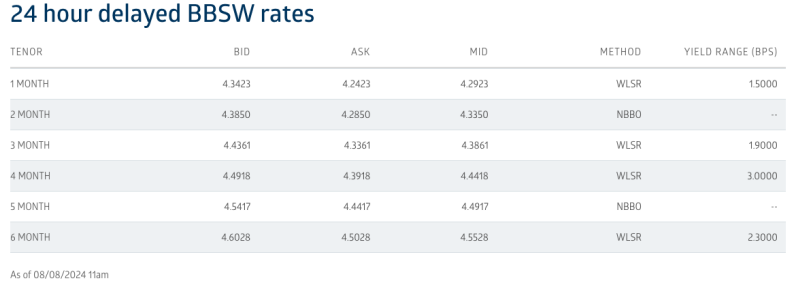
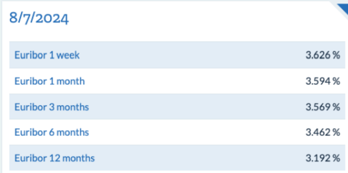
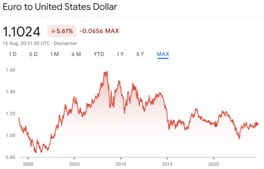
We use Python to download exchange rates and price a 3-month at-the-money EUR:USD currency option (EUR = foreign currency).

• SOFR - risk free interest rate in America
• Euribor - $r_{f}$ in Euro

SOFR	Euribor	Spot

Let’s first convert the simple Term SOFR and EURIBOR interest rates to continuous compounding. The future value of $1 invested at a simple interest rate $s$ is $1 + sT$. Under compound interest $r$, it is $e^{rT}$. Hence, for each of these rates, we want to find $r$ satisfying $1 + sT = e^{rT}$. Rearranging, we get

$$r=\frac{1}{T}\log (1+sT)$$

I calculate the continuously compounded rates to be $r_{f} = 0.03553$ and $r_{d} = 0.05071$.

import numpy as np , yfinance as yf
from scipy . stats import norm
EURUSD = yf. download (" EURUSD =X")["Adj Close "]
ret = np.log( EURUSD ).diff (1). dropna ()
sigma = np.std(ret)*np.sqrt (252)
T = 90/360; S = 1.1024; K = S # at -the - money
rf = (360/90) *np.log (1+0.03569*90/360) # Euro is the foreign currency
rd = (360/90) *np.log (1+0.0510283*90/360) # USD is the domestic currency
d1 = (np.log(S/K) + (rd -rf +0.5* sigma **2)*T)/( sigma *np.sqrt(T))
d2 = d1 - sigma *np.sqrt(T)
C = S*np.exp(-rf*T)*norm.cdf(d1) - K*np.exp(-rd*T)*norm.cdf(d2)
P = -S*np.exp(-rf*T)*norm.cdf(-d1) + K*np.exp(-rd*T)*norm.cdf(-d2)

This code gives $σ = 0.11245$ and call and put option values

In [1]: C
Out [1]: 0.0266
In [2]: P
Out [2]: 0.0225

Risk-neutral pricing and geometric Brownian motion

The ideas of risk-neutral pricing and geometric Brownian motion are central to all of quantitative finance and derivative security pricing.

• We touch on the very basics as a starting point into more advanced quantitative finance.
• We will also use both concepts for pricing options via Monte Carlo simulation in a few weeks time.

• Risk-neutral approach
  • Present some exotic options, priced with Monte Carlo techniques

It’s important to note that the Black-Scholes model is derived under a large list of assumptions. Some of these include what might be called the “usual assumptions” in financial theory and modelling:

• Constant risk-free rate $r$ and volatility $σ$ over life of option.
• No restrictions on borrowing and lending.
• Borrowing and lending rates are equal.
• No transaction costs like brokerage, bid-ask spreads, taxes, etc.
• Assets are infinitely divisible (can buy “1.0346” units).
• No restrictions on short selling.
• Trading is continuous (at infinitesimally small time intervals).
• There are no arbitrage opportunities in markets.

• Standard market modelling - Black Scholes
  • usual assumptions you come across in classical theory
  • Assumptions around people's behaviour
  • Borrowing and lending rates equal, etc.

We’re not so much interested in them as we are in the assumption on the stochastic or random process followed by the underlying asset.

• This assumption basically characterises the Black-Scholes framework and tells us the correct interpretation of the volatility parameter $σ$.
• In the risk-neutral pricing approach, we can prove that the underlying asset follows geometric Brownian motion (GBM)

$$S_{t} = Se^{(r-\frac{1}{2} \sigma ^{2})t + \sigma \sqrt{t} Z} \: \: \text{for} \: \: 0 \le t \le T$$

where $Z$ is a standard normal random variable. This implies that the underlying asset’s returns are normally distributed:

• Assumptions of the underlying asset
• Underlying assets returns are normally distributed

Rearranging the above, the asset’s continuously compounded returns

$$r_{t} = \log \frac{S_{t}}{S} = \left( r - \frac{1}{2} \sigma ^{2} \right)t+\sigma \sqrt{t}Z$$

are normally distributed with $\mathbb{E}[r_{t}]=\left( r - \frac{1}{2} \sigma ^{2} \right)t$ and Var$[r_{t}] = \sigma ^{2}t$

• This is the proper interpretation of $σ$, namely that it’s the “diffusion” parameter in geometric Brownian motion.

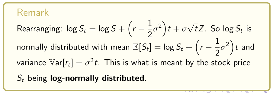
• Black Scholes pricing model assumes that the underlying asset prices returns are normally distributed
• Log of the stock price is normally distributed
  • Stock price returns are log-normally distributed

Geometric Brownian Motion

In the risk-neutral approach, the underlying asset follows geometric Brownian motion as presented above. We can simulate it as follows:

• Monte carlo approach simulates paths under geometric Brownian motion
  • Takes the actual payoff of the derivative security on the final date of European options
  • Actual price is the average of those payoffs discounted back at the risk free rate

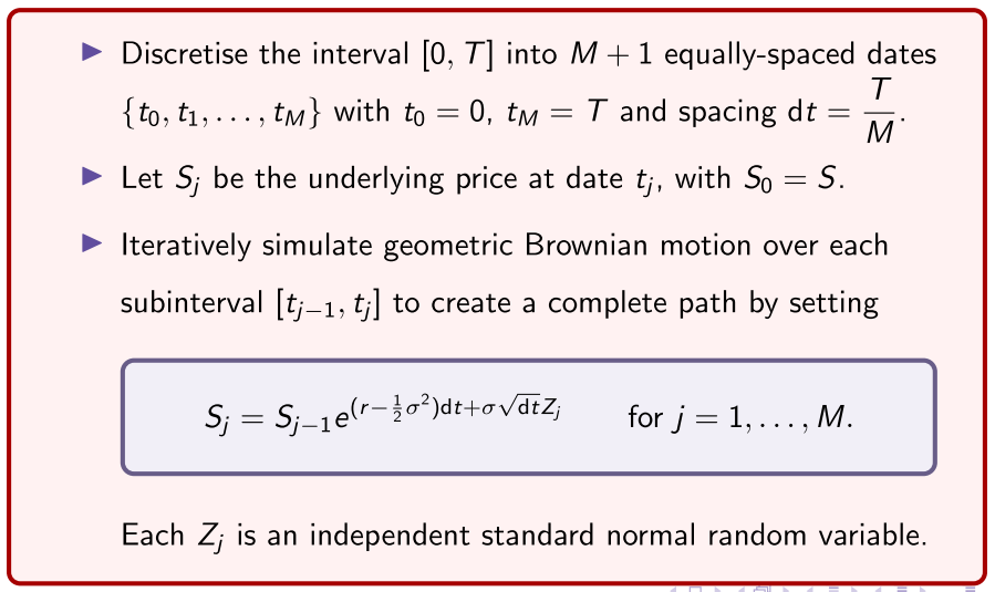
• $T_{M}$ maturity date
• Over each intermediate time interval, simulate geometric brownian motion, calculate what the underlying price of the asset is going to be
  • Each step, independently sample another draw from a standard normal random variable

Example

Simulating GBM by the above is used in the Monte Carlo simulation pricing of options, and we do this later in the course. Here is some Python code that simulates and plots geometric Brownian motion paths:

import numpy as np
from scipy . stats import norm
import matplotlib . pyplot as plt
S0 =50; r =0.05; T=1; sigma =0.25
M =1000; dt=T/M; dates =np. linspace (0,T,M+1) # 1000 time steps
N=10; S=np. zeros ([N,M+1]); S[: ,0]= S0 # 10 paths , each starting at S=50
for i in range (N):
for j in range (1,M+1):
Z=norm.rvs () # simulate outcomes of standard normal random variable
S[i,j]=S[i,j -1]* np.exp ((r -0.5* sigma **2)*dt+ sigma *np.sqrt(dt)*Z) # GBM
plt.plot(dates ,S[i ,:])
plt.title ("N=10 paths of geometric Brownian motion ") # plot

• N number of simulations (number of paths)
• j step, simulate a draw from a standard normal variable

Risk-Neutral approach

But what is meant by the “risk-neutral” pricing approach? First note:

Law of finance: The value of an asset is the present value of its expected futures cashflows or payoff.

We can use a lot of complex maths to show that the value of European options in the risk-neutral approach is given by the law of finance:

$$C = e^{-rT}\mathbb{E}[\max (0, S_{T}-K)]$$

And

$$P = e^{-rT}\mathbb{E}[\max (0, K - S_{T})]$$

where $S_{T}$ is log-normally distributed as specifi ed above.

• Value of an option is the present value of the expected future payoff
• $S_{T}$ is a random variable
  • discounted at the present value at the risk free rate
  • Don't add a risk premium

So in the risk-neutral pricing approach the value of a European option is

• the present value of its expected future payoff
• but discounted at the risk-free rate r.

Remark

So in the risk-neutral pricing approach, investors don’t add a risk premium to the discount rate, since it’s just the risk-free rate r.

• Investors are “neutral” to risk.

We can also rederive the futures/forward pricing formulas again here in the risk-neutral approach:

The payoff of a long futures contract is $S_{T} − K$, so the value of a long futures contract in the risk-neutral approach is

$$V=e^{-rT}\mathbb{E}[S_{T}-K]=e^{-rT}\mathbb{E}[S_{T}]-e^{-rT}K$$

But K is set so these contracts have 0 value: V = 0. In the risk-neutral approach, the value of every asset is the present value of its expected future payoff , including the underlying asset, so $S = e^{−rT}\mathbb{E}[S_{T}]$. So using this and rearranging the above yields

$$K=e^{rT}S$$

Variables affecting option prices and the Greeks

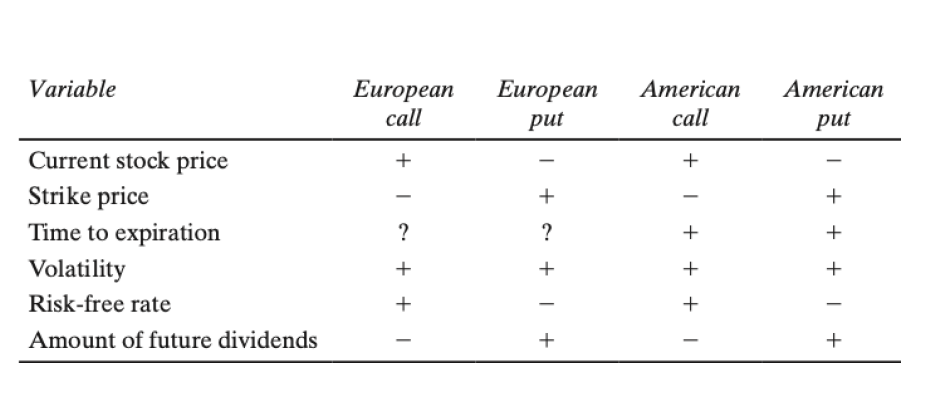
We now want to investigate and quantify how each of the input variables $K$, $S$, $r$, $T$, $σ$ and $q$ impact option premiums.

• In the Black Scholes model, a number of parameters that go into the equations
  • all parameters that can change - if we change it, how does it impact the Black Scholes option price?
• Pricing options of the market, will it make the price go up or down?
  • Trading options
• Using options so far to speculate movement in the price of the underlying asset
• use options to speculate on an increase or decrease, based on interest or volatility in the market
  • purchase options based on perceptions in the market

If you hold a derivatives portfolio

• exposed to underlying assets
• exposed to changes in interest rates, changes in time, market volatility perceptions
  • If we can quantify the impact, can create hedging strategies to insulate variable you don't want to be exposed to

The Black Scholes model

$$C = \mathcal{N} (d_{1}) − Ke^{−rT}\mathcal{N} (d_{2})$$

$$P = Ke^{−rT}\mathcal{N} (-d_{2}) - S\mathcal{N} (-d_{1})$$

(Ignoring dividends $q$ for now) where:

$$d_{1} = \frac{\log \frac{S}{K} + (r + \frac{1}{2}\sigma ^{2})T}{\sigma \sqrt{T}}$$

$$d_{2} = d_{1} - \sigma \sqrt{T}$$

depends on the variables $S$, $K$, $r$, $T$ and $σ$.

• We’re interested in the relation between them and option prices.

We know that call (put) options with a higher strike price K have lower (higher) values, and we’re not so much interested any further in K.

• want to know how these variables impact on options prices
• Don't care about options pricing with changing strike price

The Greeks

We’re interested in the sensitivity of option prices to the other variables $S$, $r$, $T$ and $σ$, and we give these sensitivities special Greek names:

• Delta ∆ is the sensitivity of the option price to S.
• Gamma Γ is another measure of the relation between prices and S.
• Rho ρ is the sensitivity of the option price to rates r.
• Vega ν is the sensitivity of the option price to volatility σ.
• Theta θ is the sensitivity of the option price to time T.

We cover each of these one-by-one.

Remark: We will assume no dividends q since the equations are neater, until right at the end where we mention the impact of dividends.

Delta ∆ and gamma Γ

We know that as $S$ increases, calls premiums rise and put premiums fall.

We quantify this mathematically with the delta ∆, given by

$$∆_{C} = N(d_{1}) \: \: \text{and} \: \: ∆_{P} = N(d_{1}) − 1$$

Importantly, note the following, which confirms the first line of this slide:

$$0 < ∆_{C} < 1 \: \: \text{and} \: \: -1 < ∆_{P} < 0$$

• $\Delta _{C}$ - change in the price of an option premium
• call option delta (how much the option premium changes from a change in the underlying asset)
• CDF of normal variable
  • As the price of the underlying asset goes up, put premium goes down

Remark ∆ is the partial derivative of the premium with respect to S

But think of ∆ as:

• The change in the premium due to a change in S.
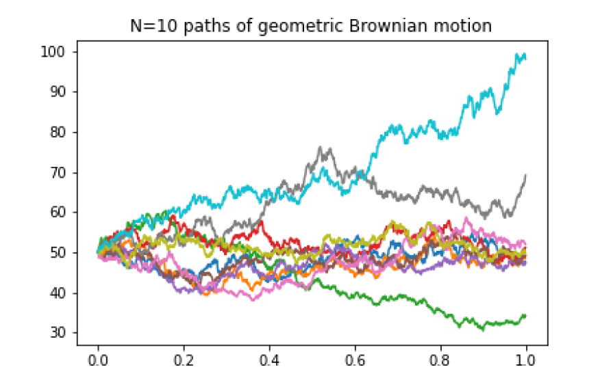
• In fact, ∆ is the slope of the above payoff diagrams:

From the remark above, we interpret ∆ as the change in the premium due to a change in S, giving us the approximations

$$dC \approx \Delta _{c} dS \: \: \text{and} \: \: dP \approx \Delta _{p} dS$$

where $dC$ and $dP$ are a change in the premium and $dS$ a change in $S$.

• We calculate the “new” premiums due to a change in S as

$$C_{new} \approx C + dC \: \: \text{and} \: \: P_{new} \approx P+dP$$

Remark: These approximations are used later in delta hedging.

• Will trade a certain quantity of the underlying asset to make their portfolio delta neutral, so that any change in the underlying asset doesn't impact on their actual value in their portfolio
• Market makers make money by quoting large spreads
  • To hedge the risk of their portfolio, changing from a change in the price of their underlying asset they will remain delta neutral the whole time
  • How many units in the underlying asset they have to trade to remain delta neutral

From above, the approximation $dC \approx \Delta _{c} dS$ is not perfect, but:

• We can make it more accurate by also using the gamma Γ given by

$$\Gamma = \frac{f(d_{1})}{S \sigma \sqrt{T}}$$

(same for calls and puts), with:

$$f(x) = \frac{e^{-x^{2} / 2}}{\sqrt{2 \pi}}$$

the PDF of a standard normal random variable

Remark: Γ is the 2nd partial derivative of the premium with respect to S.

• f notation, PDF of the standard normal variable

We make the approximations of dC and dP more accurate by setting

$$dC \approx \Delta _{c} dS + \frac{1}{2}\Gamma dS^{2} \: \text{and} \: \: dP \approx \Delta _{p} dS + \frac{1}{2}\Gamma dS^{2}$$

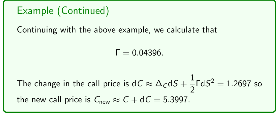
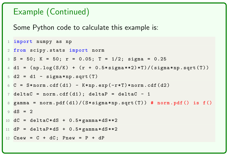
• Calculate the gamma of the call option as before
• Include the correction term
  • delta - gamma strategy

Rho $\rho$

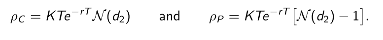
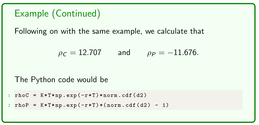
Rho ρ is the change in the premium from a change in r, and is given by

Note that:

As r increases, call premiums increase but put premiums decrease.

• An intuitive explanation for this is the present value $e^{−rT}K$ of the strike that the holder pays in a call, or receives in a put, decreases.

• $\rho$ of a call option is positive, meaning an increase in interest rate increases the value of a call option
  • Vice versa for puts

Remark: ρ is the partial derivative of the premium with respect to r.

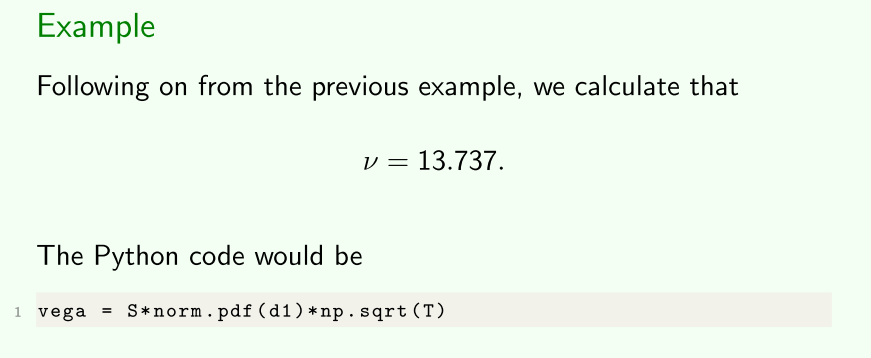
Vega $\nu$

Vega ν is the change in the premium from a change in σ, and is given by:

$$\nu = Sf(d_{1})\sqrt{T}$$

• Same for calls and puts

with f(x) the PDF of a standard normal random variable. Note that

$$0 < \nu$$

As σ increases, option premiums increase.

Remarkν is the partial derivative of the premium with respect to σ.

• As market perceptions of volatility increase, the option premiums increase
• All kinds of options strategies that you can put in place

Theta $\theta$

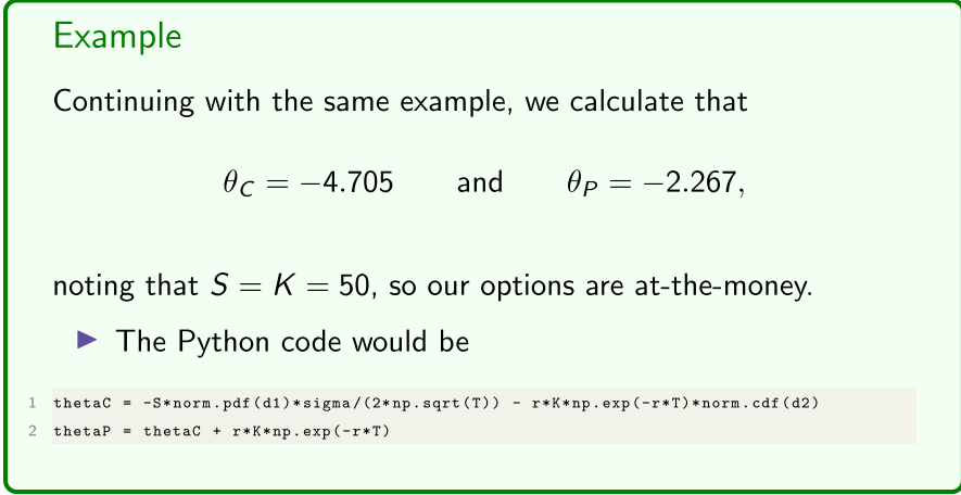
Theta θ is a bit ambiguous. It gives the negative of the change in the premium from a change in T. And the equations are more complex:

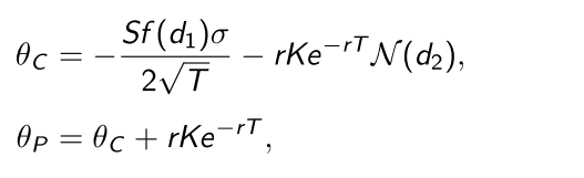
with f (x) the PDF of a standard normal random variable.

• consider the case of option on income-paying options
  • can be positive or negative, depending on the params in the market at a given point
• All of the other variables of the option price don't change

Remark θ is the negative of the partial derivative of the premium with respect to T, telling us the impact of approaching expiry.

However, note that

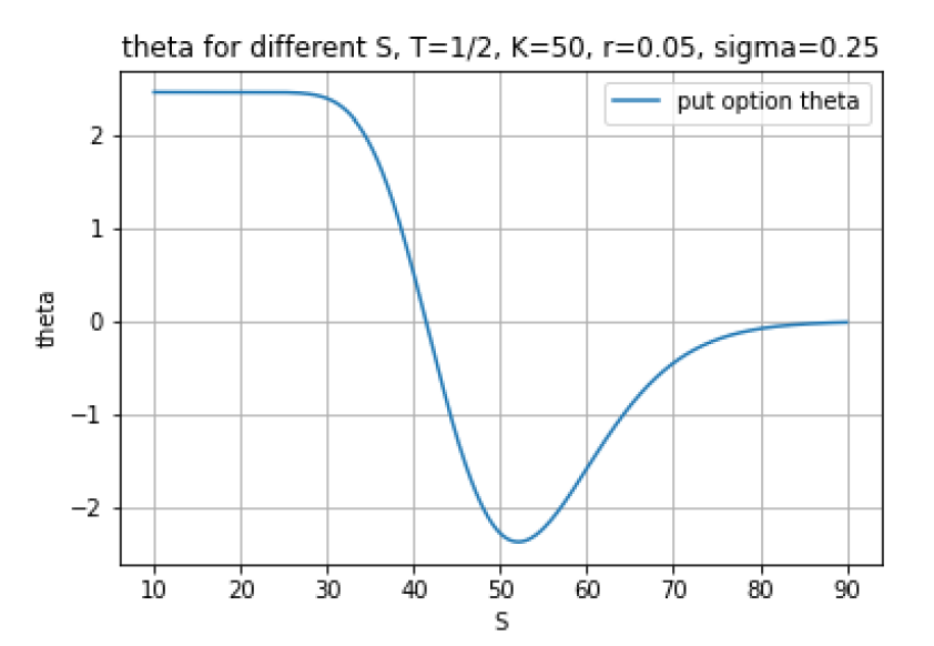
On a non-dividend paying asset, call premiums fall as expiry nears.

• Impact of time on puts is ambiguous: From $\theta _{P} = \theta _{C} + rKe^{-rT}$ deep in-the-money put (large K) premiums may increase as expiry nears.
• This relates to something said last week: A deep in-the-money put is already close to its maximum payoff of K, so not much more payoff can be realised at expiry, but there is still a chance of an unfavourable movement in the asset price. But as we approach expiry, there is less chance of an unfavourable movement.

However, there is some rules of thumb relating to time:

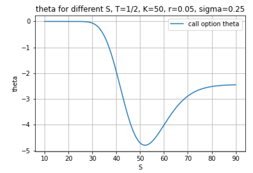
• θ is almost always negative:
• So premiums usually fall as expiry approaches.
• This is known as time decay.
• Time decay works for option writers and against option holders.
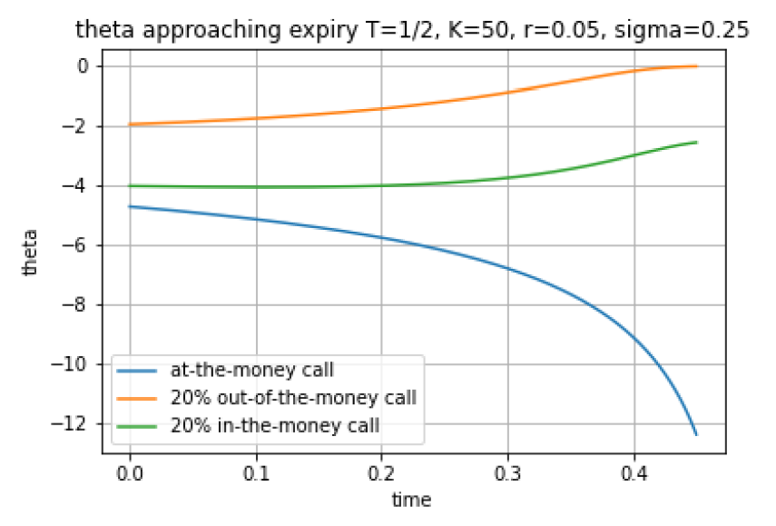
• θ is most negative for options close to at-the-money.
• θ in fact gets more negative for options close to at-the-money as expiry approaches: Time decay “speeds up” as expiry approaches. These last two points are illustrated in the following fi gures:

• Always assume that $\theta$ is negative for calls and puts

  • Core premium falls no matter what, as you approach expiry, given all other param stay the same

• non-dividend and dividend paying assets could put premiums

• Ignoring small percentage of cases, all other options have negative theta

  • Always assumes your premiums are falling as you approach expiry
  • Time decay

• Portfolio of long options, portfolio is going down in value as you approach expiry

  • Write an option, receive the premium upfront
  • Premium time value approaches zero - take advantage of time decay that works for you
  • More impactful as you approach expiry

• options with trading positions close to the money

Incorporating dividends

On a dividend paying asset, all of the above interpretations remain unchanged except for θ. From the textbook, the equations become:

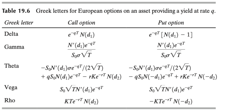
Note that Hull uses the notation N′(x) for the PDF of a standard normal random variable, whereas I’ve been using f(x).