Lecture 6

Delta Hedging and Delta-Gamma Hedging

Last week we presented the basics of the Black-Scholes model for European options on non-income paying assets, income paying assets, and currencies. We also presented the Greeks, which quantify the relation between option premiums and the Black-Scholes model input parameters.

This week we look at delta hedging, which is a common strategy employed by traders and market makers to manage risk and is the starting point for other “Greek neutral” strategies. We then cover the notion of implied volatility and fi nish with using the concepts of the Greeks, delta hedging and implied vols to present some basic trading strategies.

• Readings: Chapters 12, 15.11, 19.4 and 20 of Hull.

• exam mostly about intuition and finance theories
• How money makes make money

Static delta hedging

• We start off with the basic idea of static delta hedging.

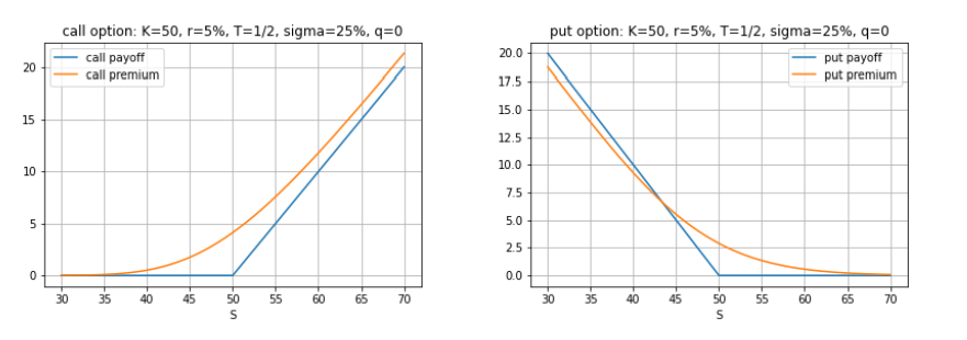
Recall the basic long call and put option payoff and premium plots:

• trying to hedge the risk of changes in the underlying asset
• at the money call option
  • orange is the premium of the option
  • Using black scholes pricing
• If the asset price goes up/down

Delta hedging

• how many units in the stock should I take to hedge this risk?

Static delta hedging

An option’s delta is an approximation of the change in the premium due to a change dS in the price S of the underlying asset:

$$dC ≈ ∆_C dS \; \; \text{and} \; \; dP ≈ ∆_P dS.$$

We use an option’s delta to hedge a position against changes dS in S:

Delta hedging involves taking a position in the asset to hedge an option position against small movements in the asset’s price.

So, given an option position, we calculate how many units Q in the asset we need in order to hedge against small changes dS in the asset price S.

• Negative Q means a short position in the asset.

• Money makers options in the market
  • take an advantage of one of the greeks
  • closely hedged to changes in price to the underlying asset
  • only want to be exposed to certain of the other parameters that go in as an input to the Black Shoals

Delta hedging

• How many units (what trade in the underlying asset) in order to hedge in changes against the price in the underlying asset
• need to hold a negative amount in the underlying asset

Static delta hedging

The value of a portfolio of $h = 1$ call option and Q units in the asset is

$$V = QS + C$$

The change $dV$ in $V$ due to a change $dS$ in $S$ is given by

$$dV = QdS + dC$$

$$\approx QdS + ∆CdS = (Q + ∆ C )dS$$

• Q units in the underlying asset
• how many units of Q so that the change in our portfolio doesn't change

Remark The value of a portfolio of h = 1 put option and Q units in the asset is $V = QS + P$ and its change is

$$dV ≈ (Q + ∆ P )dS$$

Delta hedging means choosing Q so that dV = 0.

• From the relations

$$dV = (Q + ∆_C )dS \; \; \text{and} \;\; dV = (Q + ∆_P )dS$$

to set $dV = 0$ we easily see that Q should be chosen to equal

$$Q ≈ −∆ C \; \; \text{or} \;\; Q ≈ −∆ P$$

Remark Setting $Q$ to the above so $dV = 0$ means we’re delta neutral.

• hold a call option and it goes up
  • go short in the asset
• put option
  • go long in the asset

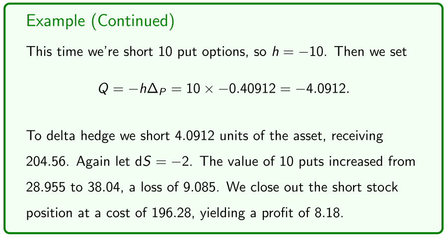
We can generalise delta hedging to a portfolio of h > 1 options:

Static delta hedging

The value of a portfolio of $h$ calls and $Q$ units in the underlying asset is

$$V = QS + hC$$

and its change in value is

$$dV = QdS + hdC$$

$$≈ QdS + h∆_C dS = (Q + h∆_C )dS$$

To be delta neutral, so $dV = 0$, we set $Q = −h∆_C$.

Remark The value of a portfolio of $h$ puts and $Q$ assets is $V = QS + hP$. Its change is $dV ≈ (Q + h∆_P )dS$ so we set $Q = −h∆_P$ .

• typically hold more than one option

• Did not make the hedge perfectly
  • ignoring the gamma of the option
  • Price of an option over a range of asset prices is actually curved
  • Gamma tells us the curvature

Remark

We’re assuming assets are “infinitely divisible”. Options contracts are typically over $m$ assets (the multiplier). Then the portfolio values are $V = QS + hCm$ or $V = QS + hPm$ with changes

$$dV = (Q + h∆_C m)dS \; \; \text{or} \;\; dV = (Q + h∆_P m)dS$$

So for delta hedging we round $Q = −h∆_C m$ or $Q = −h∆_Pm$ to whole numbers, which doesn’t “badly damage” the hedge.

We can use gamma $\Gamma$ to improve delta hedging:

Delta-gamma hedging

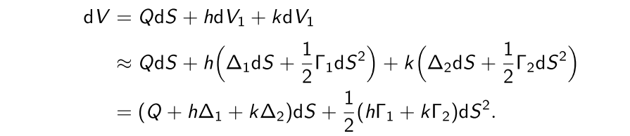
Recall from last week that we can make our approximations of the changes dC and dP in option premiums due to a change dS in the underlying asset price S more accurate by including Γ as follows:

$$dC ≈ ∆_C dS + \frac{1}{2}ΓdS^2$$

$$dP ≈ ∆_P dS + \frac{1}{2} ΓdS^2$$

We can use delta-gamma hedging to improve the delta hedging of an option position by taking a position in the asset and a different option.

• takes into consideration convexity
• delta hedging, position in the option
• delta gamma hedging, need a position in the stock and another option

Delta-gamma hedging involves taking a position in the asset and in another, different option to hedge an existing option position against small movements in the price of the underlying asset.

So, given a position of h options, for delta-gamma hedging we calculate how many units $Q$ in the asset and $k$ in another option we need in order to hedge against small changes $d$S in the price $S$ of the underlying asset.

The value of a portfolio of $Q$ units in the asset, $h$ units of one option, and $k$ units of another, different option is given by

$$V = QS + hV_1 + kV_2$$

where $V_1$ and $V_2$ are the respective option premiums.

Also let $∆_1$ and $Γ_1$ be the delta and gamma of our existing option, and $∆_2$ and $Γ_2$ be the delta and gamma of the new option.

The change in portfolio value approximated by delta-gamma hedging is

NOTE: typo (should be $kV_2$)

So when setting $dV = 0$, for delta-gamma hedging we need to solve

$$Q + h∆_1 + k∆_2 = 0$$

and

$$hΓ_1 + kΓ_2 = 0$$

Remark Solving these equations for $Q$ and $k$ so that $dV = 0$ means that we’re both delta and gamma neutral.

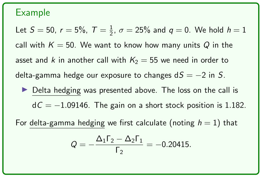
We can show that the solution is

$$Q = -h \frac{\Delta _1 \Gamma _2 - \Delta _2 \Gamma _1}{\Gamma _2}$$

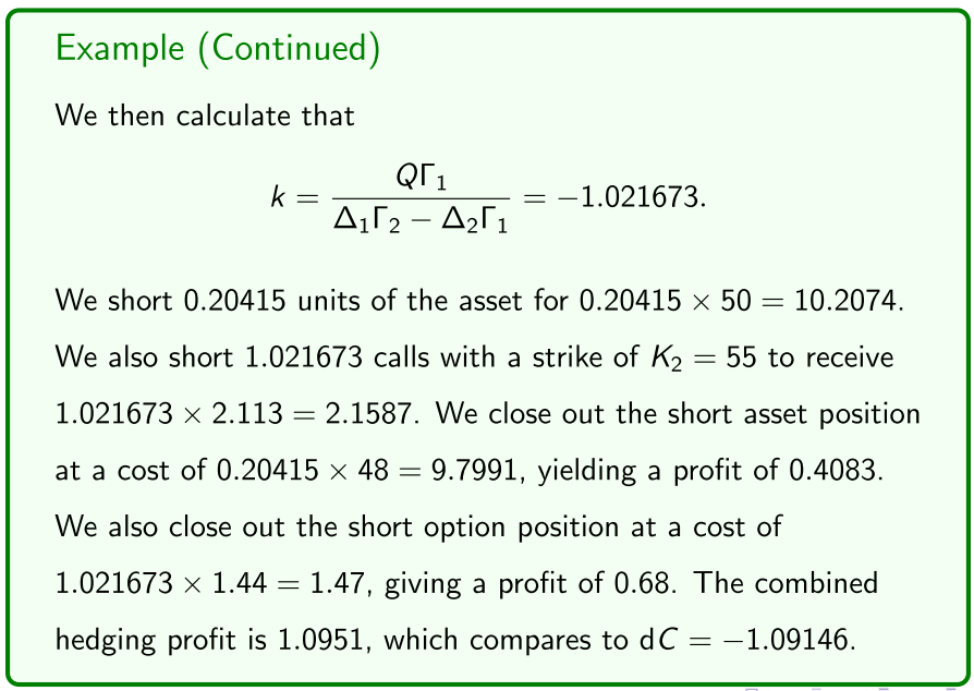
And

$$k = \frac{Q \Gamma _1}{\Delta _1 \Gamma _2 - \Delta _2 \Gamma _1}$$

So to delta-gamma hedge an existing option position, we use the first equation to calculate $Q$ and then the second equation to calculate $k$.

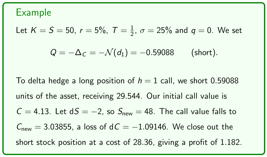
• Consider the previous example of long $h = 1$ call:

Dynamic delta hedging

So far we’ve been doing “1 period” delta hedging.

• But when the asset price S changes, so does the option’s delta.
• Hence, to stay delta hedged over time, one needs to regularly rebalance the holding Q in the underlying asset.
• We also rebalance our bank account as we buy and/or sell the asset.
• And pay and/or receive interest as appropriate.

Dynamic delta hedging involves maintaining a “rolling” delta hedge (staying delta neutral) over time via regular rebalancing.

An example best illustrates the idea, in which we use daily rebalancing.

• Did an example instantaneously

• one period, one point in time hedge

• at regular intervals, quickly delta hedge so not exposed to what happens overnight

  • maintaining/rolling regular delta hedging
  • delta changes after a particular interval
  • as the price of the options changes, so does your delta

• At regular points an time, compound forward the interest that we paid for too

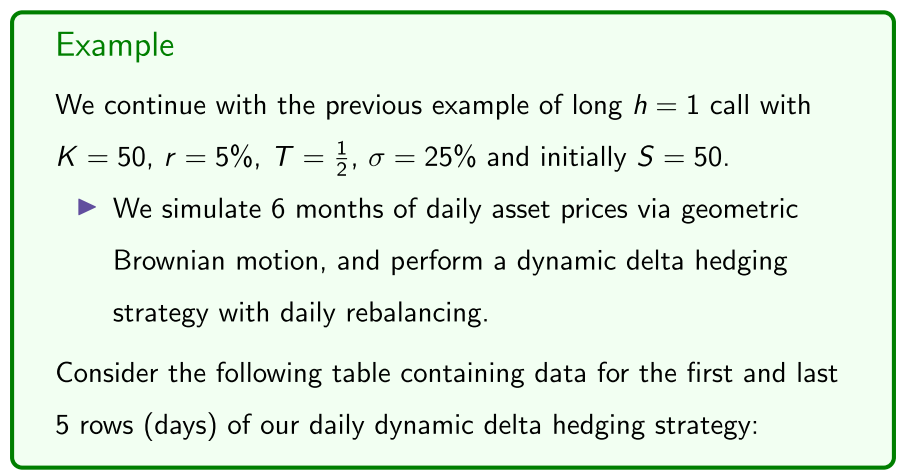
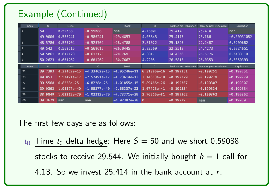
• S, price of the asset at the end of the first day
• delta of the option (column 2)
• Q how many units in the underlying asset I need to hold
• Stock, value of the stock multiplied by the quantity of the units I need to hold in the stock
• Bank ac pre-rebalance - how much money we have in the bank account pre-rebalancing
• Bank ac post-rebalance - if we continued the delta hedging strategy

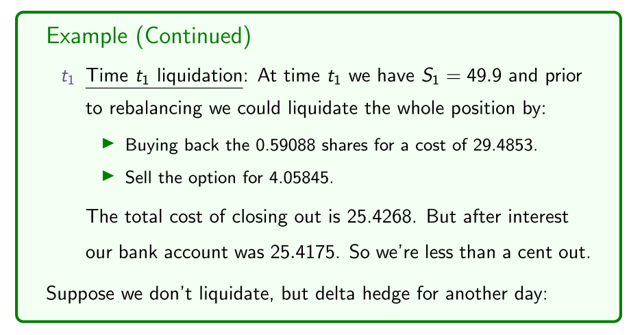
• sell option for 4.05845, considering one less day till expiry the cost 29.4853m
• earn interest from the first day, from 25.414 to 25.4175

Remark We can make this delta hedging process more accurate by:

• Using a shorter time period: Say delta hedging every hour.
• Use another option and do dynamic delta-gamma hedging.

Also note that in reality dynamic hedging is not as “neat and clean” as this due to market imperfections such as bid-ask spreads, brokerage fees, different borrowing and lending rates, etc.

• rebalancing only every day, not hour, e.g.
• hedge an option position to changes in the underlying asset
• market imperfections make this a lot less favourable

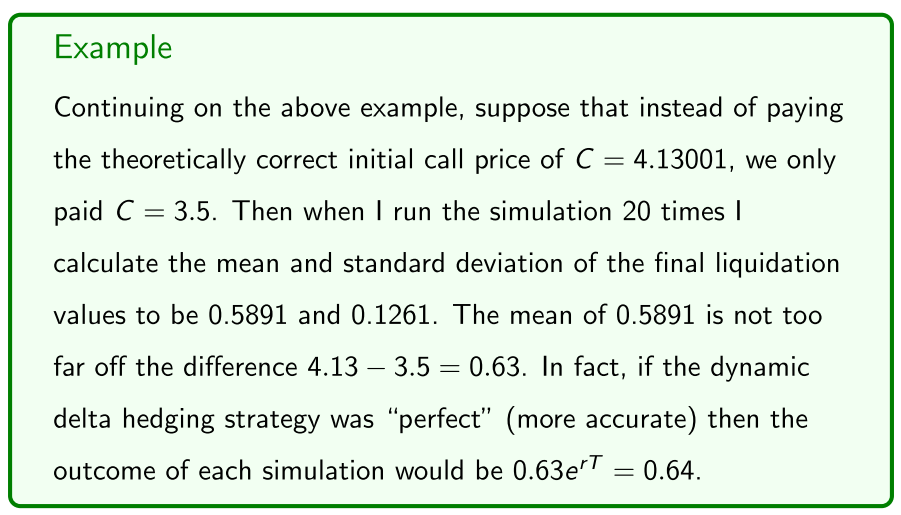
Note also that in the above, we assumed that we initially bought the h = 1 call for the theoretically correct Black-Scholes value.

Question: How do market makers make money?

One way market makers make money is by their bid-ask spread and hence trading options at a “more favourable” price than the theoretically correct price, and then dynamically delta-hedging to “lock in” their profi t.

• Consider the following example:

• Market makers; make a market for someone to trade at
  • Offer the bid/ask spread
  • they trade at the favourable side of the spread
  • make their money by trading at the more favourable price of the bid/ask price
• Every time someone does a trade, they can lock in their spread

• ASSIGNMENT NOTE, 1:14:00

Implied volatility

We now turn to the “mysterious” and “elusive” volatility parameter σ in the Black-Scholes model.

In the Black-Scholes European option pricing model

$$C = S\mathcal{N} (d_{1}) − Ke^{−rT}\mathcal{N} (d_{2})$$

$$P = Ke^{−rT}\mathcal{N} (-d_{2}) - S\mathcal{N} (-d_{1})$$

Where

$$d_{2} = d_{1} - \sigma \sqrt{T}$$

$$d_{2} = \frac{\log \frac{S}{K} + (r -\frac{1}{2}\sigma ^{2})T}{\sigma \sqrt{T}}$$

the only unobservable parameter is the volatility σ.

• We’ve been estimating it using historical data but traders use market conventions, their knowledge of the market and even intuition when determining the volatility parameter σ to use for pricing options.

Here, we’re interested in calculating σ from option prices:

• $\sigma$ is the annualised volatility in the underlying asset

• previously lecture, based on historical data

  • not done by traders, use intuition

• point of the parameter is what traders are forecasting the asset to show over the life of the asset

• can work backwards, knowing all the other parameters used to price options

  • determine the implied volatility

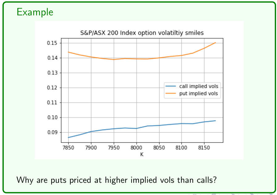
Across the different range of strike prices, higher for options out of the money versus in the money

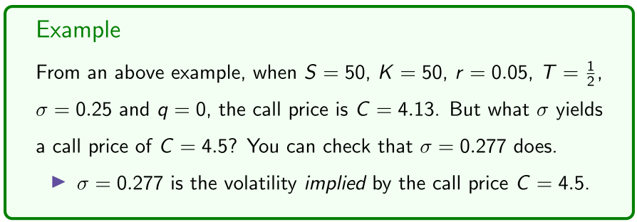
Given observed option prices C or P and observable market vari- ables S, K, r and T, an option’s implied volatility is the volatility parameter σ that yields Black-Scholes prices equal to C or P.

The question is: How do we calculate implied vols?

There’s no “nice and neat” equation to calculate implied vols.

• We have to code numerical (iterative) techniques on computers. I don’t go into the mathematical details but I’ll give you some Python code to calculate implied vols using Newton’s method.

import numpy as np; from scipy . stats import norm
# function to calculate Black - Scholes option prices
def black_scholes (S, K, r, T, sigma , q):
d1 = (np.log(S/K) + (r - q + 0.5* sigma **2)*T)/( sigma *np.sqrt(T)); d2 = d1 - sigma *np.sqrt(T)
C = S*np.exp(-q*T)*norm.cdf(d1) - K*np.exp(-r*T)*norm.cdf(d2) # call
P = -S*np.exp(-q*T)*norm.cdf(-d1) + K*np.exp(-r*T)*norm.cdf(-d2) # put
return [C, P]
# function to calculate option vega
def vega(S, K, r, T, sigma , q):
d1 = (np.log(S/K) + (r - q + 0.5* sigma **2)*T)/( sigma *np.sqrt(T))
return np.exp(-q*T)*S*norm.pdf(d1)*np.sqrt(T) # same for calls and puts
# observed call or put price
obs = 4.5 # call price , change for put price
# known / observed / given parameter values
S = 50; K = 50; r = 0.05; T = 1/2; q = 0
# Newton ’s method
sigma = np.sqrt (2* np.abs(np.log(S/(K*np.exp(-r*T))))/T) # initial guess of sigma
val = black_scholes (S, K, r, T, sigma , q)[0] # call price , change to [1] for puts
while (abs(val -obs) >10** -8):
v = vega(S, K, r, T, sigma , q)
sigma = sigma - (val - obs)/v # Newton step to update / improve estimate of sigma
val = black_scholes (S, K, r, T, sigma , q)[0] # call price , change to [1] for puts
print (" implied volatility =", sigma )

In markets, Black-Scholes implied vols are not constant but display:

• A volatility smile or smirk over the range of strike prices.
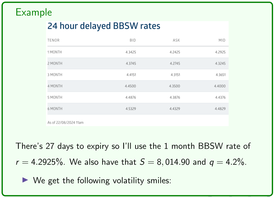
• A volatility term structure over the range of expiry dates. Lets calculate some implied vols from S&P/ASX 200 Index option quotes.

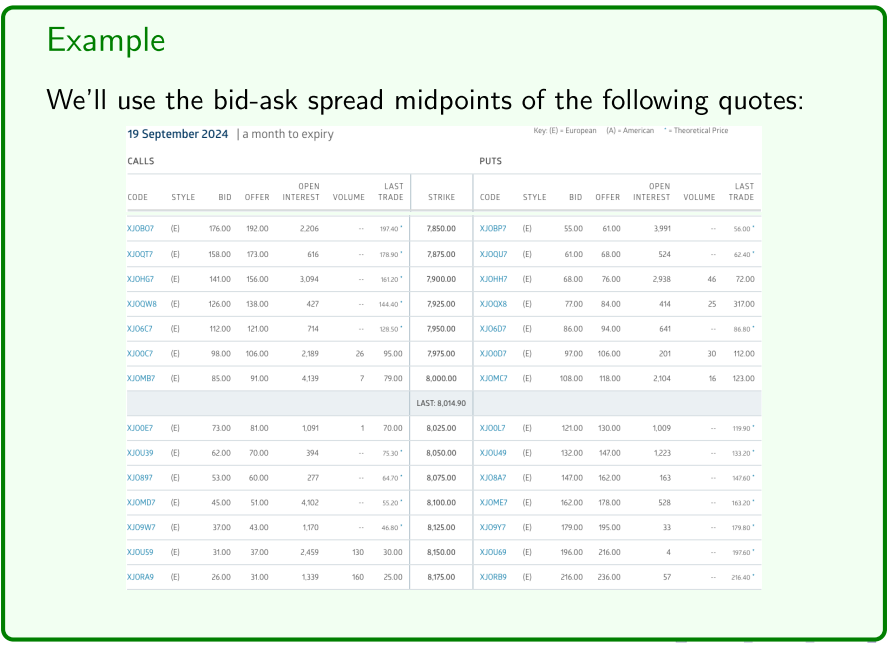
• Black scholes volatility params

VIX index

• The Cboe VIX Index measures “market wide” implied vols:

It “is a calculation designed to produce a measure of constant, 30-day expected volatility of the U.S. stock market, derived from real-time, mid-quote prices of S&P 500 Index (SPX) call and put options.”

• See here for a detailed explanation, plus wiki and Investopedia.

The Cboe VIX index is effectively an average of the implied volatilities of a large range of 30 day Cboe S&P 500 Index options.

• One can even trade futures and options on the VIX (also see here)!

• estimates of implied volatilities

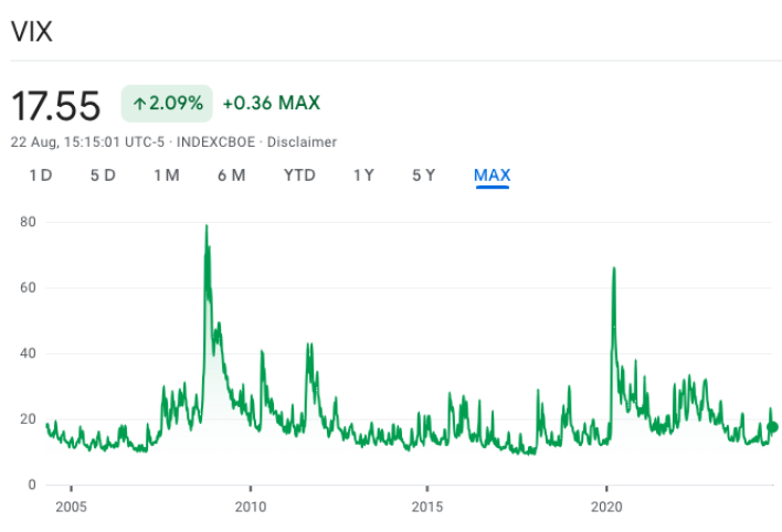
A value of 17.55 means that average implied vols of 30 day S&P 500 Index options, thus the market’s 30 day volatility expectations, is 17.55%.

• varies everyday, based on sentiment of the market

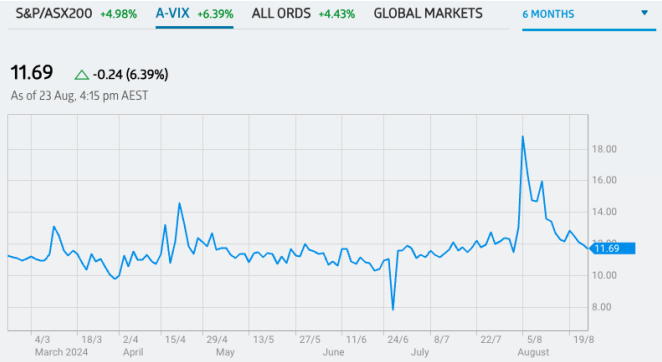
The implied vol of the S&P/ASX 200 Index is quite a bit lower at 11.69 than that of the S&P 500 Index of 17.55, and is roughly “in the middle” of our above S&P/ASX 200 Index option volatility smile and smirk.

• 11.69, in the middle from the put/calls volatilities
  • 30 day options (puts and calls)

As an observation, the VIX index tends to spike when the market falls:

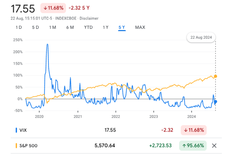
• spiked massively in COVID

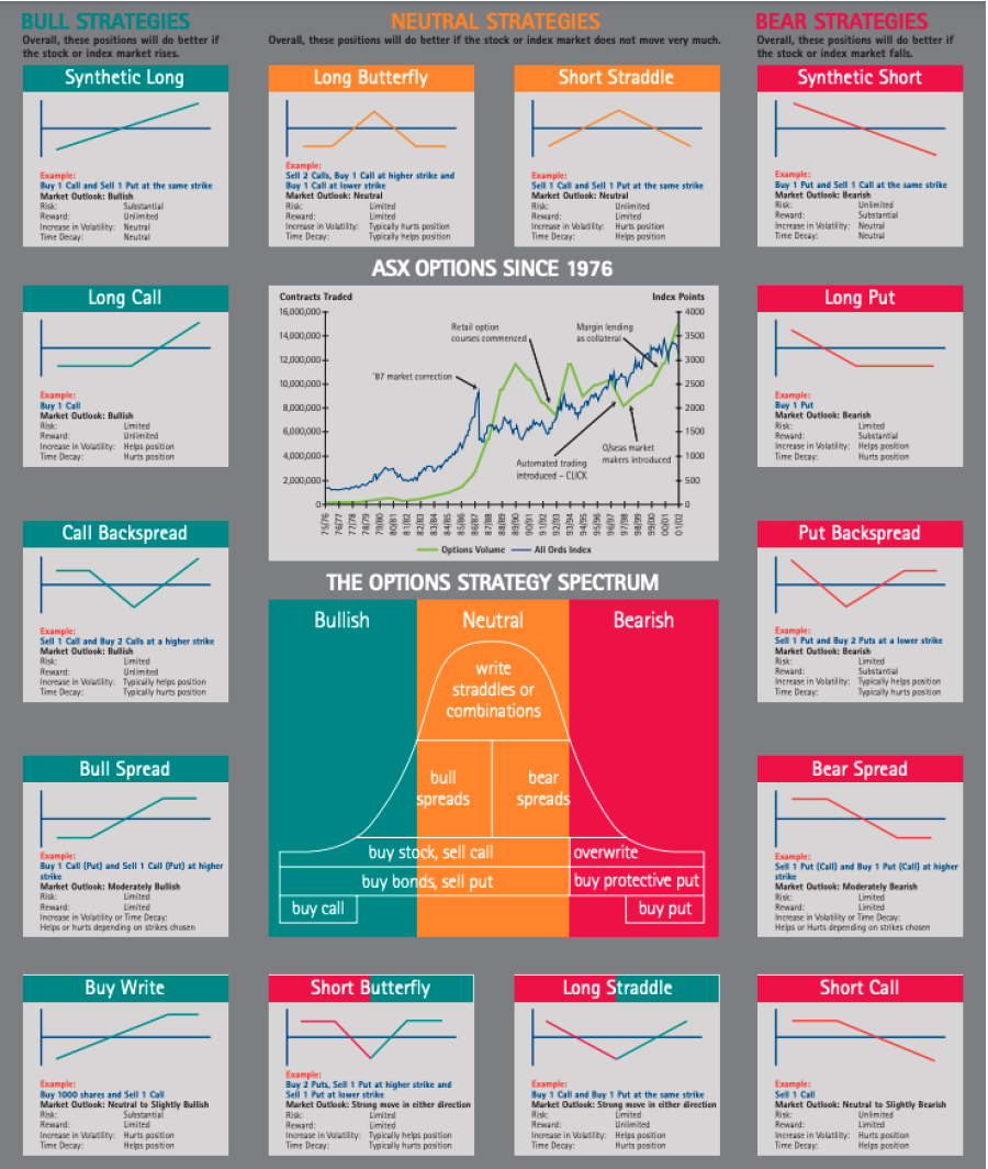
Trading strategies

We now present some “standard” options trading strategies designed to take advantage of movements in the asset price, changes in market sentiment and implied vols, and the passage of time:

• Directional strategies: Speculate on the direction of the price of the underlying asset, similar to taking calls and puts.
• Volatility strategies: Speculate on high or low asset volatility, or changes in implied vols, often incorporating delta neutrality.
• Time: Strategies that seek to take advantage of time decay, typically assuming low asset volatility and relatively constant implied vols.

• Trading strategies, take advantage of

Remark We’ve already present some basic options strategies, including:

• Taking calls (puts) to speculate on an increase (decrease) in the price of the underlying asset.
• Covered calls or a “buy-write” involving writing calls on a portfolio of the underlying asset.
• Portfolio insurance, involving taking puts over a portfolio of the asset in order to protect it against market falls.

• Portfolio insurance - Bill Ackman

It’s common to divide trading strategies into two different classes:

• Spreads: Positions in the same type (call alone or puts alone) of options on an asset, but with different strikes and possibly expiries.
  • Bull and bear spreads.
  • Backspreads and ratio spreads.
  • Butterfly and condor spreads.
  • Calendar spreads.
• Combinations: Positions in both puts and calls on an asset.
  • Straddles and strangles.
  • Butterfly and condor combinations.
  • Strips and straps. The payoffs of many strategies can be created in different ways, and we can create strategies containing both spread and combination positions

• Options portfolio

Directional strategies

Directional strategies seek to speculate on a directional change in the price of the asset, but at a lower upfront cost to the basic strategies of taking calls and puts, while still maintaining limited downside risk.

• However, in lowering the upfront cost relative to taking calls and puts, these strategies sacrifice some upside potential, as we will see.

• asset needs to move a lot, a lot of fees associated with it
• sell an option slighting out of the stock to reduce fees

Suppose we want to speculate on an increase in the asset price:

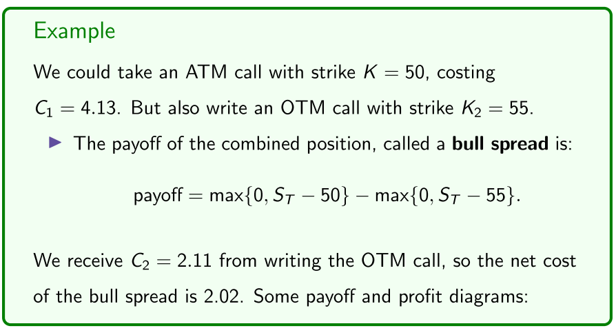
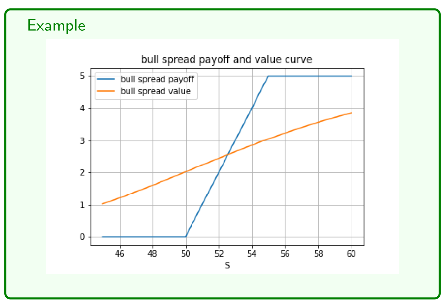
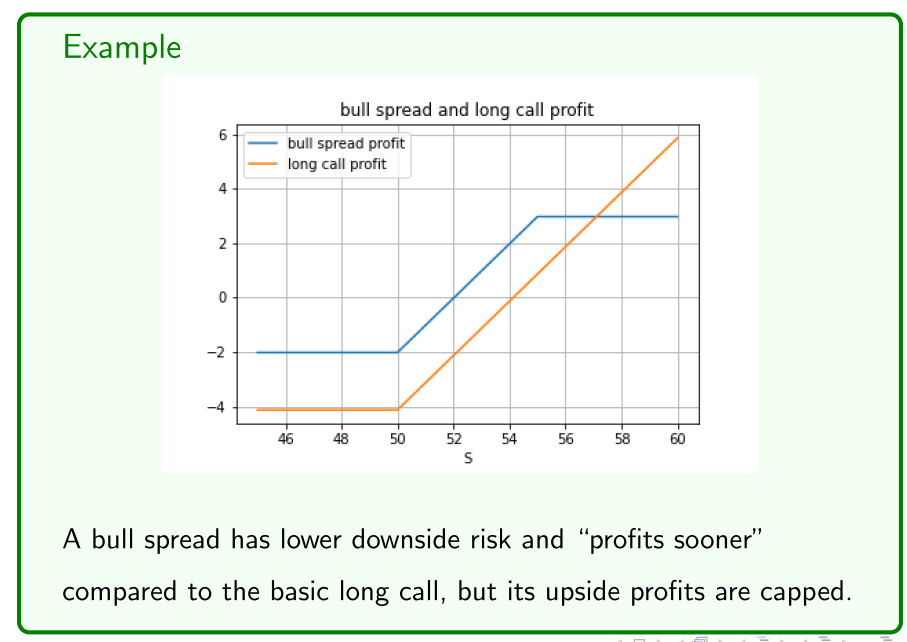
• bull spread doesn't cost us as much initially
  • earn a profit earlier, but payoff gets capped

Remark Bull spreads can also be constructed from puts (tutorial question).

Now suppose we want to speculate on a decrease in the asset price:

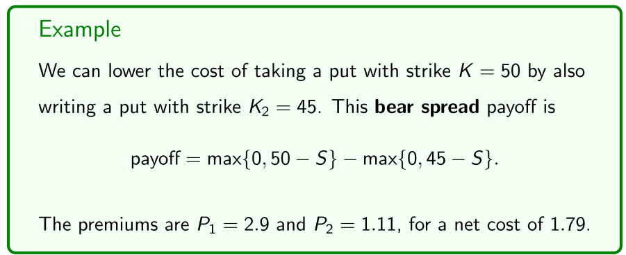
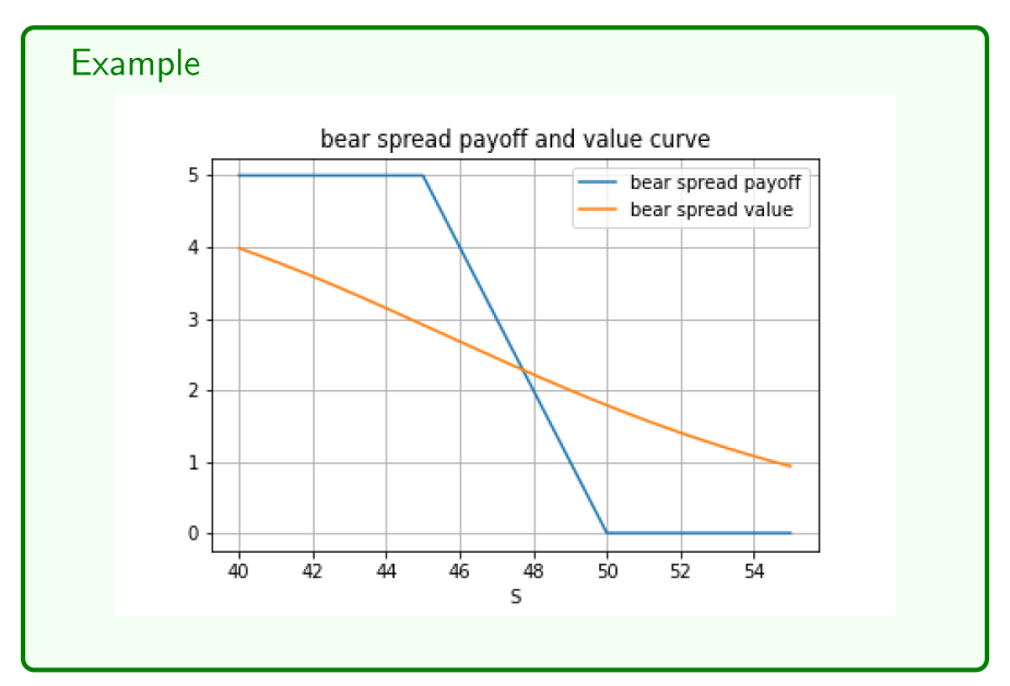
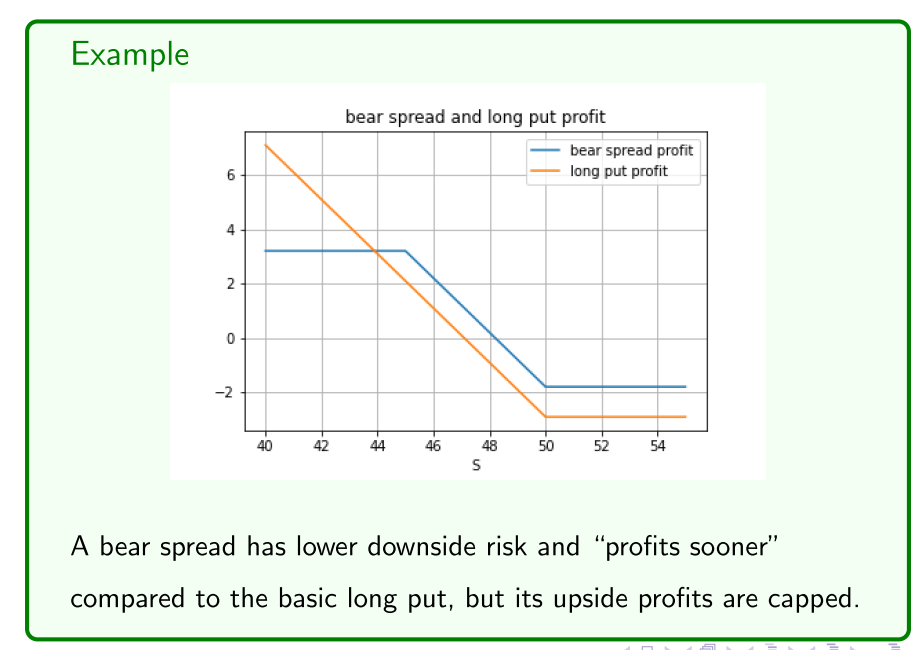
• cost us less, start to make a profit sooner

The basic strategies of taking calls, as well as bull and bear spreads, seek to speculate on the asset price moving in a given direction.

• But what if we think the asset price will be very volatile but we’re not sure about which direction it will go?
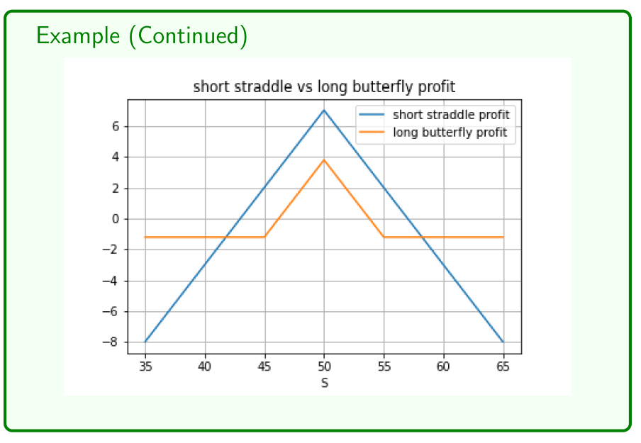
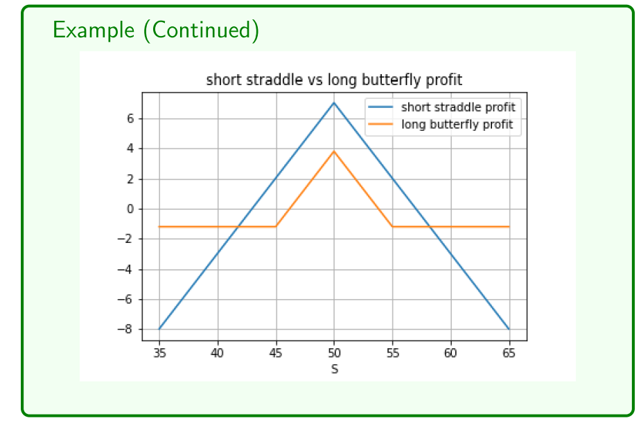
• Also, what if we think the asset price will be stable?

How might we trade options given these views or beliefs?

Volatility strategies

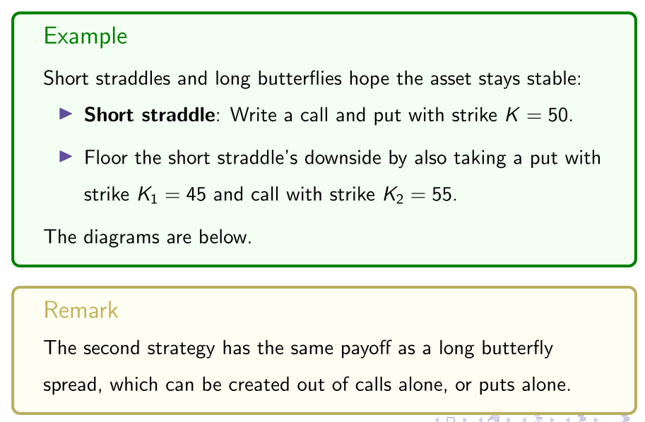
Volatility strategies seek to take advantage of the asset either staying stable or displaying high volatility. Another class of volatility strategies also seek to take advantage of changing market sentiment and hence implied vols, while typically staying delta (and possibly gamma and theta) hedged. They’re best described with examples.

• Suppose we think that the asset price will be volatile:

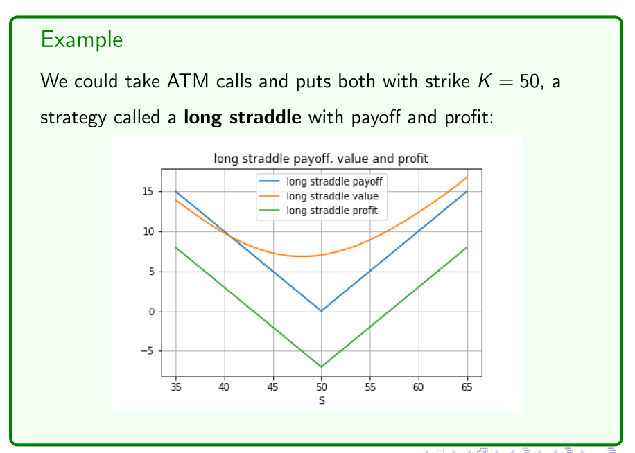
• orange, value of the put plus the value of the call
• payoff, is minus whatever the premium costs

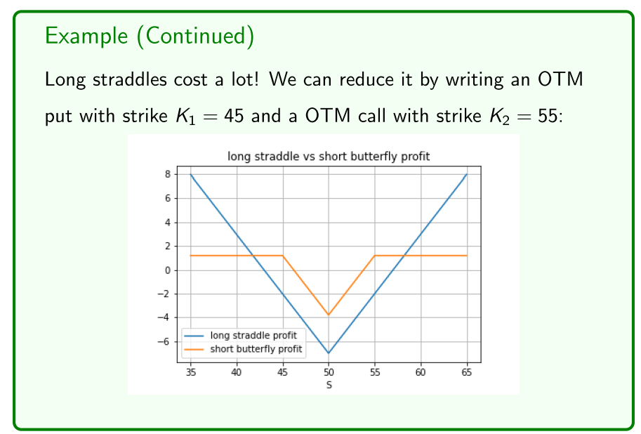
• Cap the payoff, and shift to reduce the premium

The above strategies are all just speculating on the asset price, as are: