Lecture 7

European calls and puts are relatively simple plain vanilla derivatives.

• In this simple context we can derive a nice, clean Black-Scholes equation or formula for their premiums:

$$C = Se^{-qT}\mathcal{N} (d_{1}) − Ke^{−rT}\mathcal{N} (d_{2})$$

$$P = Ke^{−rT}\mathcal{N} (-d_{2}) - S e^{-qT}\mathcal{N} (-d_{1})$$

Where:

$$d_{1} = \frac{\log \frac{S}{K} + (r - q + \frac{1}{2}\sigma ^{2})T}{\sigma \sqrt{T}}$$

$$d_{2} = d_{1} - \sigma \sqrt{T}$$

The Black-Scholes European call and put option pricing model results in an analytical or closed-form solution equation or formula.

• volatility parameter
• black scholes model assume volatility parameter is constant
• analytical/closed form solution
• In quant finance that rarely happens

1. When applying the Black-Scholes framework to derive pricing models for more complex, exotic derivatives (even just for American options), we immediately run into the scenario of being unable to derive closed-form, analytical solution equations.
2. We may also want to apply more complex derivative security pricing frameworks than the Black-Scholes framework (say the Heston stochastic volatility, or the Merton jump-diffusion, frameworks), but again we immediately run into the same problem.

• pricing plain vanilla options,
• want to price much more complicated securities
• may depend on values for the underlying asset
  • want to price much more complex derivative securities
  • no actual equation or solution

Extended models

• If we apply these different pricing models, might not be able to create an equation

Numerical methods:

Question: How do we proceed in these scenarios of trying to

1. price complex derivative securities and
2. use more complex derivative security pricing frameworkswhen we can’t derive a closed-form solution equation or formula?

Answer: We use numerical approximation or computational techniques:

• We use computers and iterative algorithms.

Remark These numerical algorithms are similar to Newton’s method for the IRR of a bond or implied vol of an option.

• called numerical approximation techniques
• code to determine the applied volatility of an option
• Use numerical computation techniques

Three main numerical or computation approaches:

1. Lattice type methods like the binomial and trinomial models.
2. Monte Carlo methods:

• Motivated by the risk-neutral approach to derivative security pricing.

3. Partial diff erential equation numerical solution methods:

• Motivated by the partial diff erential equation (PDE) approach to derivative security pricing (we avoid it in FINM3405).

In FINM3405 we focus on the binomial and Monte-Carlo methods.

• Numerically solving PDE is a too messy mathematically.

• lattice type method, use an iterative technique to determine the price of an asset
• Mostly use mote-carlo method
  • easy to parallelize
• Partial differential equation approach
  • derive a partial differential equation
  • Use numerical schemes to solve PDE

Question: Why do we require more complex derivative security pricing frameworks than the Black-Scholes framework?

Answer: When calibrated to market data, the Black-Scholes framework does not accurately price observed options trading in the market.

• when estimating the volatility in the black scholes model

Remark We see this from the volatility smile and term structure:

• The volatility parameter σ we need to use to get the Black-Scholes model to match observed option premiums is not constant across the range of strike prices and expiries.

• Is more art than science
• From a more scientific perspective, using more complex pricing models

Consequently traders use:

• Rules of thumb, intuition and market conventions and experience to determine the σ parameter to use in the Black-Scholes model.
• Other, more complex and accurate option pricing models.

Remark
Calibrating an option pricing model means estimating the unobserved input parameters of the model using statistical techniques. In the Black-Scholes model the only unobservable parameter is the volatility σ. Due to the assumption of geometric Brownian motion, the maximum likelihood estimator of σ is the annualised standard deviation of the underlying asset’s historical returns. But using this estimate for σ in the Black-Scholes model results in inaccurate option prices, as we’ve seen.

The reason that the Black-Scholes model, when using the maximum likelihood estimator of its unknown parameter σ, does not accurately price observed options in the market is that the Black-Scholes model is derived based on a large list of very restrictive and unrealistic assumptions. The two main assumptions important to us are:

1. The underlying asset’s returns are normally distributed, or equivalently, the asset’s price is log-normally distributed.
2. The volatility parameter σ is constant over the life of an option. These two assumptions do not hold in reality:

• unrestrictive and unrealistic assumptions
• Historical returns are normally distributed
• The volatility parameter is constant

The below plots display common stylised features of fi nancial returns:

• Non-normality:
  • Spiked mean.
  • Narrow shoulders.
  • Fat tails.
  • Skewness, or at least extreme negative return events.
• Volatility clustering or regimes (non-constant volatility).

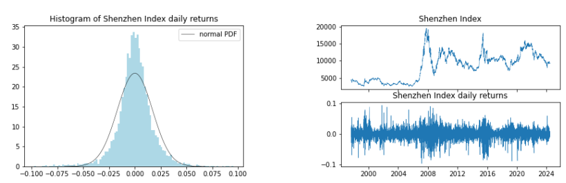
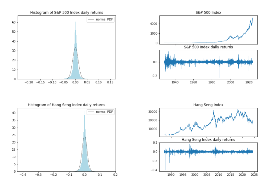
• assumption of normality in financial markets doesn't hold
• financial market returns are not normally distributed
• main reason why black Scholes doesn't work very well

A significant amount of research in quantitative fi nance involves developing (i) more complex and accurate option pricing models and (ii) models that are able to price more complex, exotic options.

• Relating to (i), a particular focus of this research is deriving option pricing models in which the underlying asset is assumed to follow a random process that matches or models observed asset price returns more accurately than geometric Brownian motion.
  • The Heston stochastic volatility model allows non-constant volatility.
  • The Merton jump-diffusion model allows jumps in asset prices.

More complex option pricing models nearly always require numerical pricing methods, so we start with basic numerical methods this week.

• Developing more complex models
• Other option pricing models based on different kinds of random processes that better model the styled features of financial markets
• Heston stochastic and Merton jump try and be more specific

American options (next week) we need to use numerical methods

binomial model

As per the Black-Scholes model, the binomial model is a pricing framework defined by a set of simplifying assumptions:

Assumptions of the 1-period binomial model

• One trading period of length $T$ years to the option’s expiry.
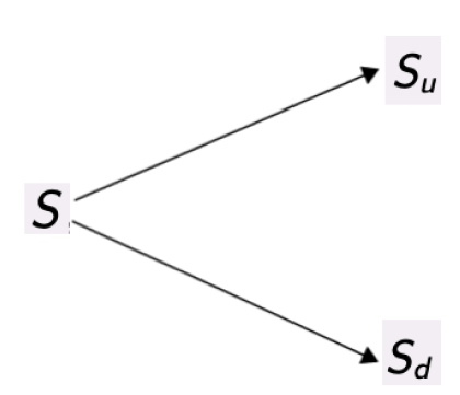
• Starting at S, two possible outcomes for the underlying asset:
  1. Up to $S_u = Su$, where $u$ is the asset’s up factor.
  2. Down to $S_d = Sd$, where $d$ is the asset’s down factor.
• A risk-free rate r satisfying $d < e^{rT} < u$.
• All the other “usual” assumptions.

• other assumptions, unlimited buying/borrowing power
• no bid-ask spreads, no transaction fees, etc.

The call option’s payoffs in each possible outcome of the price of the underlying asset are:

$C_u = \max(0, S_u − K)$

$C_d = \max(0, S_d − K)$

Figure: Possible outcomes of the price of the underlying asset.

We now use arbitrage arguments to derive an equation

$$C = e^{−rT} [qC_u + (1 − q)C_d]$$

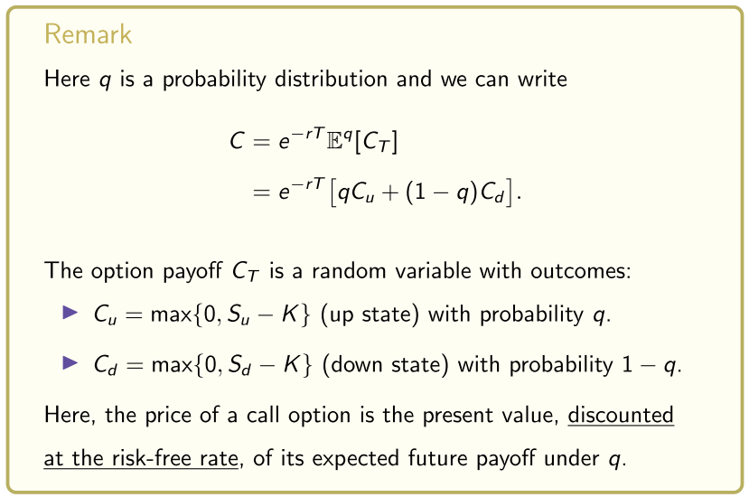
for the price C of a call option in the 1-period binomial framework, where

$$q = \frac{e^{rT} - d}{u-d}$$

is a probability distribution also derived below and that has important interpretations in quantitative finance: It is risk-neutral.

• probability distribution $q$

We set up a replicating portfolio R by investing:

• ϕ units (dollars) in the risk-free rate.
• ∆ units (hence ∆S dollars) in the underlying asset.

The replicating portfolio’s payoff s in each outcome of the underlying are

$$R_u = ϕe^{rT} + ∆S_u \;\;\;\text{and} R_d = ϕe^{rT} + ∆S_d$$

and by “replicating” we mean $R_u = C_u$ and $R_d = C_d$.

• outcome - future value at risk free rate
• replicating portfolio - 'setup a portfolio that replicates the payoff of the call option'
• Can show that the replication portfolio exists and is unique
• Trying to get this portfolio to replicate the payoffs

Remark We initially invest $R = ϕ + ∆S$ dollars in the replicating portfolio.

We can show that there is a unique replicating portfolio given by

$$\phi = \frac{uC_d - dC_u}{(u-d)e^{rT}}{(u-d)e^{rT}}$$

and

$$\Delta = \frac{C_u - C_d}{S(u-d)}$$

Remark: This replicating portfolio can be found by writing the conditions $R_u = C_u$ and $R_d = C_d$ as and then solving the linear system

$$\begin{bmatrix} e^{rT} & Su \\ e^{rT} & Sd \end{bmatrix} \begin{bmatrix} \phi \\ \Delta \end{bmatrix} = \begin{bmatrix} C_u \\ C_d \end{bmatrix}$$

The payoffs of the replicating portfolio equal those of the call option, so:

Law of one price: The replicating portfolio and call option must have the same price, otherwise an arbitrage opportunity exists:

$$C = ϕ + ∆S$$

• because we can setup a replicating portfolio, price must be the same today by law of one price

Inserting the above values for ϕ and ∆ and then rearranging, we get

$$C = e^{-rT}[qC_u + (1-q)C_d]$$

where

$$q = \frac{e^{rT} - d}{u-d}$$

and

$$1-q = \frac{u-e^{rT}}{u-d}$$

• based on some sort of expectation

By the risk-neutral world we mean quantifying the probability of outcomes in financial markets via a risk-neutral probability q.

• The value of every asset is the present value, discounted at the risk-free rate r, of its expected future cashfl ows under q.

We discount the expected future cashflows with r:

• We don’t add a risk-premium to the discount rate. This also holds for the underlying asset: We can also show that $S = e^{-rT}\mathbb{E}^q[S_T]$, where $S_T$ is a random variable with outcomes $S_u$ with probability $q$ and $S_d$ with probability $1 − q$.

• assume working with an at the money option
• up factor 1.1, can go up 10%
• typo, = should be -

Determine up and down factors

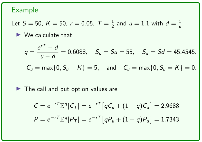
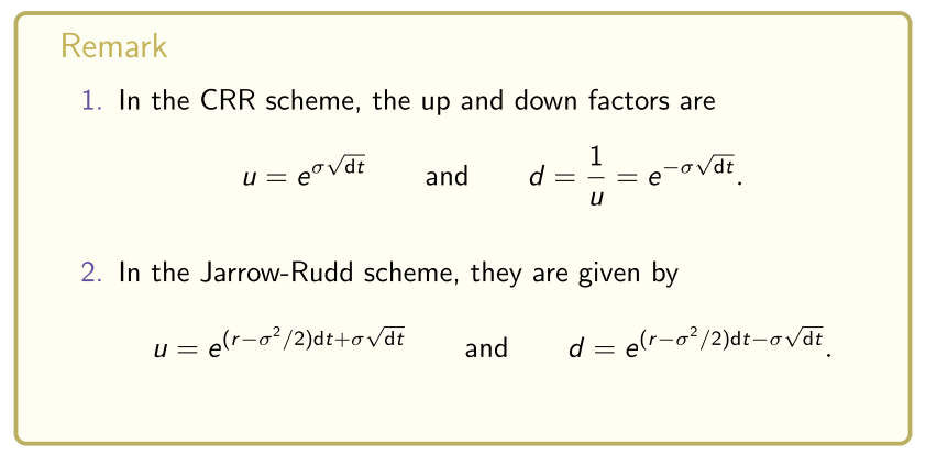
Question: Where do we get the up u and down d factors from?

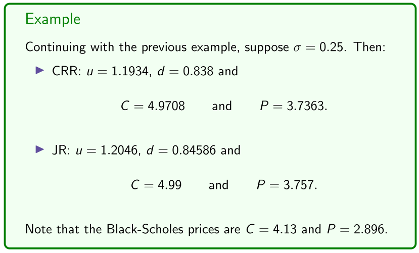
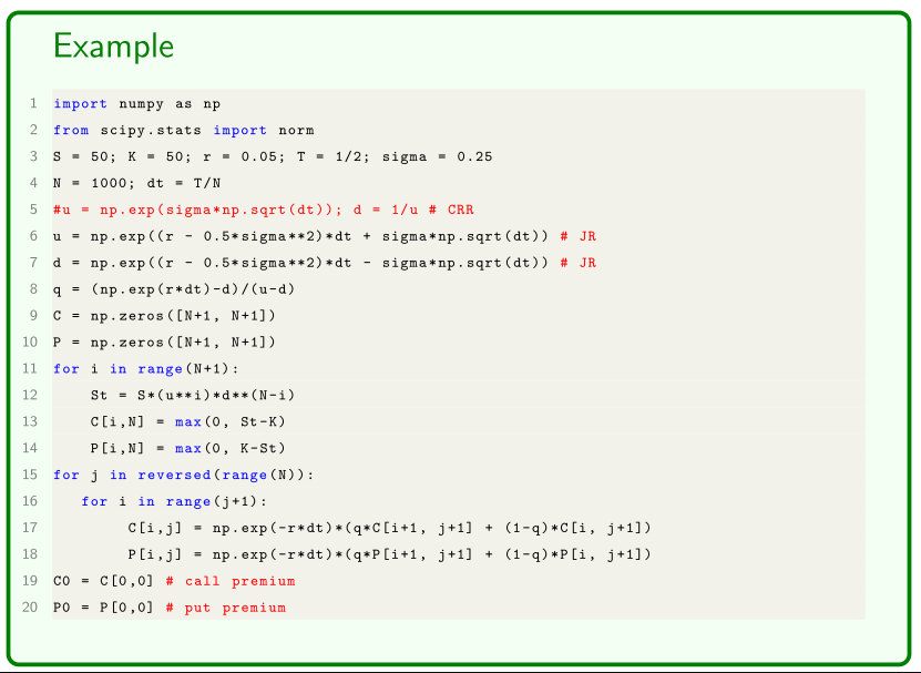
1. The Cox, Ross, Rubinstein (CRR) scheme derives

$$u=e^{\sigma \sqrt{T}} \;\;\; \text{and} \;\;\; d = \frac{1}{u} =e^{- \sigma \sqrt{T}}$$

where σ is the volatility parameter.

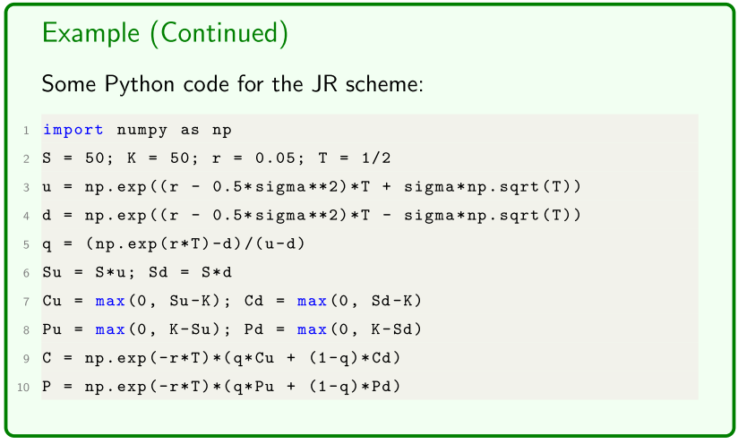
1. The Jarrow-Rudd (JR) scheme derives

$$u=e^{(r - \sigma^2 /2)T + \sigma \sqrt{T}} \;\;\; \text{and} \;\;\; d = e^{(r - \sigma ^2 / 2) T - \sigma \sqrt{T}}$$

More general and complex schemes have also been proposed.

Multi-period

For the multi-period binomial model we simply:

1. Discretise the interval [0, T] into N + 1 equally-spaced dates ${t_0 , t_1 , . . . , t_N }$ with $t_0 = 0, t_N = T$ and spacing $dt = T/N$.
2. Build an asset price tree starting at $S$ as per the next slide.
3. Calculate the option premium by recursively stepping backwards in time in the tree and using the 1-period pricing formula each step.

• work back from the previous nodes
• using one period binominal to work back in the tree - recursively step back in the tree

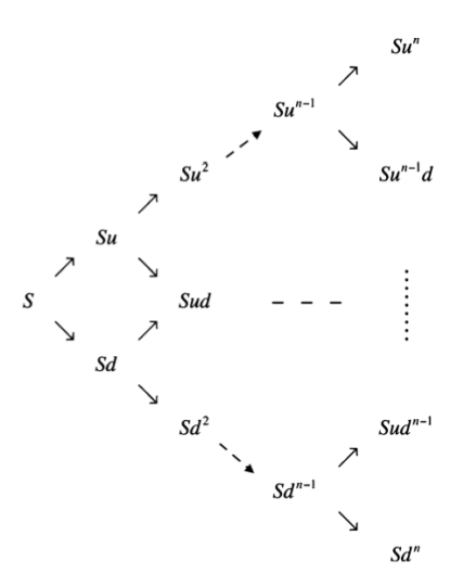
To build the asset price tree, we note that the asset price can go up by a factor of u or down by a factor of d at each time step.

• We build the asset price tree as follows:

At expiry (time T) there is N + 1 underlying asset prices

• $S_{iN} = Su^id^{N-i}$ for $i = 0, 1, . . . , N$. Asset price S$_{iN}$ took $i$ up steps and thus $N − i$ down steps.
• At time step $j$ there is $j + 1$ asset prices $S_{ij} = Su^i d^{j−i}$ for $i = 0, 1, . . . , j$. Asset price $S_{ij}$ took $i$ up steps and thus $j − i$ down steps.

• $S_{ij}$ - j records what layer we are at

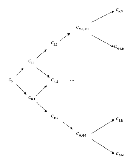
We calculate call prices as follows:

• The call option payoff s at expiry (time T) are $C_{iN} = \max{0, S iN − K}$ for $i = 0, 1, . . . , N$.
• We let $C_ij$ denote the call price at time step $j$ when the underlying asset took $i$ up steps (and thus j − i down steps)

• every single call option

• Then working backwards, starting with the expiry payoffs $C_{iN}$ for $i = 0, 1, . . . , N$, we recursively calculate the call prices $C_{ij}$ using the 1-period binomial pricing formula as follows:
  • Suppose we want to calculate the call price $C_{ij}$ at time step $j$.
  • From the previous iteration in the recursion, we know the call prices C_{i+1,j+1} (up step) and $C_{i,j+1} (down step) at time step $j + 1$.
  • We calculate $C_{ij}$ as follows:

where the risk-neutral probability is given by

• need to know how to price an option by recursively stepping back through the tree
• Need an algorithmic approach

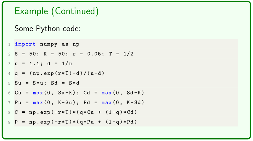
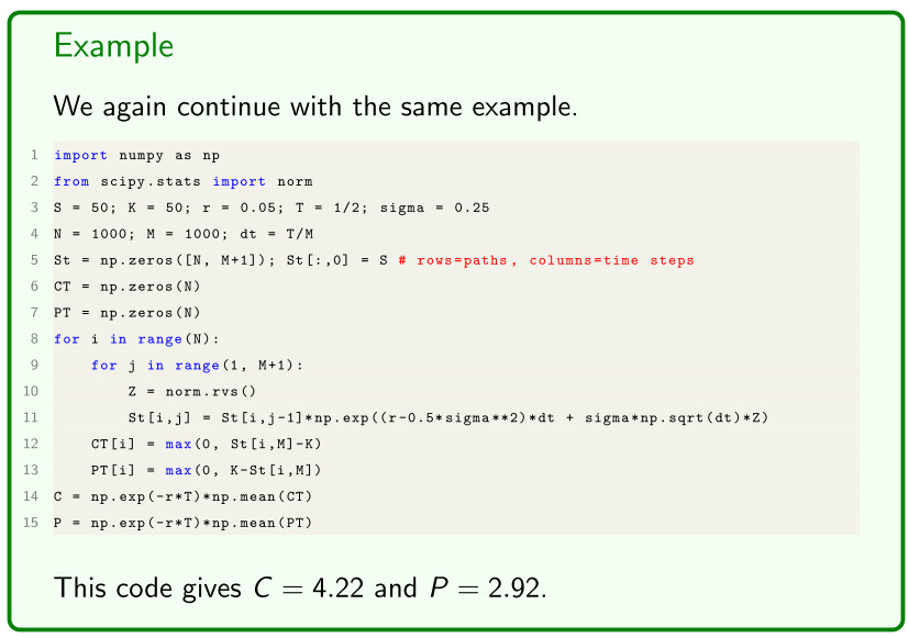
Example

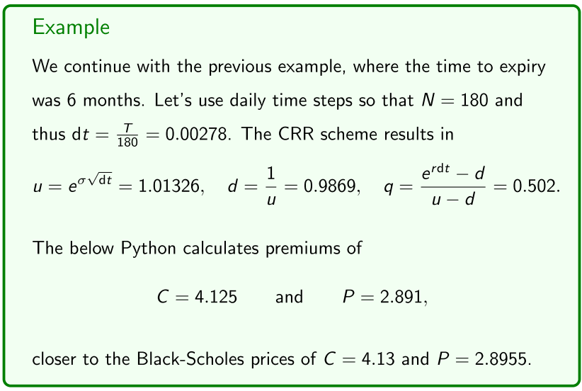
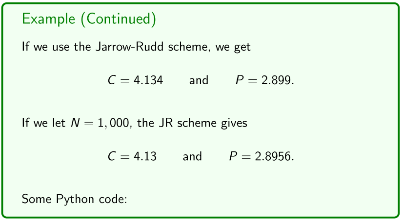
• N is too large, computer cannot handle the precision

The binomial model is useful in some option pricing contexts, such as for American options (although the PDE approach is preferred here), but the Monte Carlo approach is beneficial in other option pricing contexts.

• useful for American options, but often not used

Monte Carlo Method

The Monte Carlo method is motivated by the risk-neutral approach:

• The underlying asset follows geometric Brownian motion

$$S_t = Se^{(r - 1/2 \sigma^2)t + \sigma \sqrt{t}Z} \;\;\; \text{for} 0 \le t \le T$$

• simulate a bunch of paths in geometric brownian motion

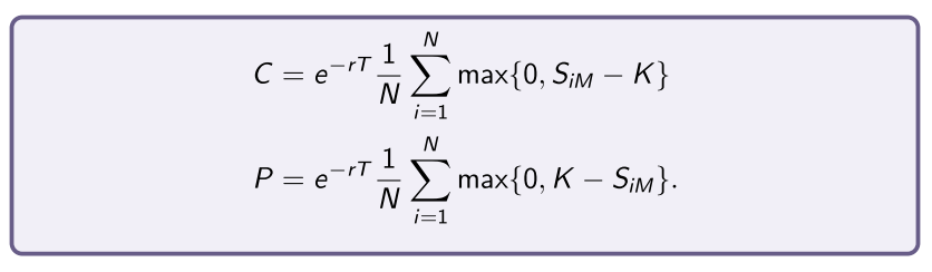
• Option prices are given by

where S T is log-normally distributed as per geometric Brownian motion.

• To price options via the Monte Carlo method we:

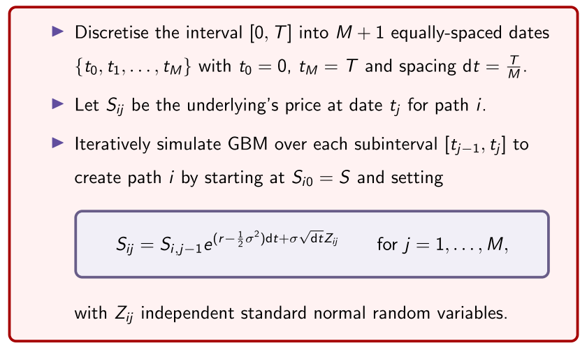
• Simulate N sample paths of geometric Brownian motion of length M + 1 as per next slide to get N asset prices S iM for i = 1, . . . , N.

• Option prices are then given by

• simulate a bunch of paths (N)
• whole bunch of final asset values
• Price is the average of payoffs, discounted back to PV using the risk free rate (see formula)

Geometric Brownian motion

Recall that we simulate geometric Brownian motion (GBM) as follows:

• M + 1, M is the number of dates
• simulate a whole bunch of asset prices, to determine the final price of the option

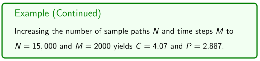
• increase the number of paths to increase precision
• generally not as good as the binomial approach
• techniques to make the conte-carlo more powerful
• applied over more scenarios

Remark There’s a number of variance reduction techniques (and vectorised and parallel coding) that make Monte Carlo methods much more accurate, powerful and computationally efficient.