FINM3405 Revision

Lecture 2-3 Futures & forwards

• 1. Definitions
  • 1.1. differences
  • 1.2. payoff diagrams
• 2. Margin mechanism and leverage effect for futures.
• 3. Calculate the value of a futures/forward contract.
• 4. The following for the main classes of futures and forwards in terms of the underlying asset, namely commodities, equities, currencies and interest rates (FRA and BAB futures):
  • Main contracts and their specifications.
  • Perfect hedging examples.
  • Basic examples of speculating on the price of the underlying asset.
• 5. Contract pricing via the cost of carry approach.
  • 5.1. Cost of Carry Futures
  • 5.2. Cost of Carry FX Contract Pricing
  • 5.3. Cost of Carry FRA Contract Pricing
• 6. Basis risk and optimal hedging.
  • 6.1. Basis Risk
  • 6.2. Optimal Hedging

Aside: Notation

• Hypothetical time interval $[0, T]$.
  • Time $t = 0$ is a contract’s initiation date.
  • Time $T$ is a contract’s maturity or delivery date.
  • Time $t$ is some intermediate date: $0 ≤ t ≤ T$.
• $S_{t}$ is the underlying asset’s spot price at time $t$.
• $K_{t}$ is the contract price at time $t$.
  • We write $S = S_{0}$ and $K = K_{0}$ to reduce notation.
• $m$ is the contract multiplier.
• $F_{t} = K_{t} \times m$ is the notional or face value of 1 contract.
• $h$ is the number of contracts we enter into.
• $K_{t}$ is the contract price when initiating a contract at time $t$.
  • Long position at time $t$: Agree buy the asset for $K_{t}$ at maturity $T$.
  • Short position at time $t$: Agree sell the asset for $K_{t}$ at maturity $T$.

Cost of Carry

• $I$ is the time $T$ capitalised interest paid on a loan used to buy the underlying asset at time $t = 0$.
• $J$ is the time $T$ capitalised storage cost of owning and holding the underlying asset from time $t = 0$ to time T.
  • Transport, warehouse storage, insurance, maintenance, etc.
• $D$ is the time $T$ capitalised dividends or other income or benefits received from owning the asset up to time T. Let
• $r$ be a simple annual interest rate,
• $s$ be a simple annual storage rate, and
• $q$ be a simple annual dividend (or later convenience) yield.

1. Definitions

• Futures and forwards are contracts between two parties to trade an agreed quantity $m$ of an asset for an agreed contract or forward price $K$ on an agreed future delivery or maturity date $T$.

1.1 Differences

The basic difference between futures and forward contracts is:

• Futures are traded on exchanges (and other trading venues).
• Forwards are negotiated directly between market participants OTC.

This has a number of implications, including:

• Contract standardisation.
• Centralised counterparty.
• Counterparty risk.
• Trading liquidity and ability to close out positions.
• Holding to maturity vs closing out early.
• Margin mechanism and daily settlement (futures only)

1.2. Payoff Diagrams

The payoffs at maturity from 1 contract (over 1 asset) are:

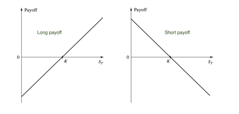
long payoff = $S_{T} − K$ and short payoff = $K − S_{T}$

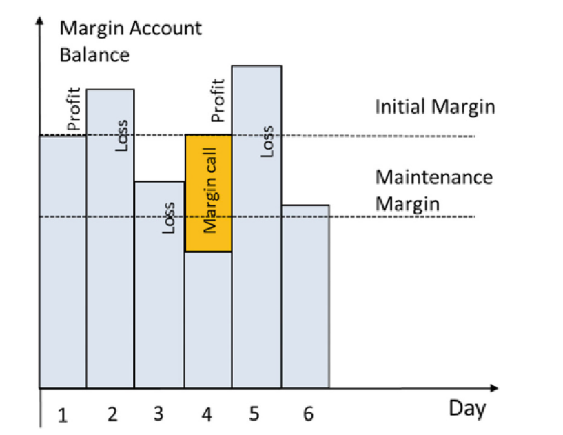
2. Margin Mechanism & Leverage Effect

The futures margin mechanism can be described as follows:

• You post an initial margin into your margin account, which is a percent of the contract price $K$ (per contract).
• Your position is marked to market on a daily basis, with daily gains (losses) credited to (debited from) your margin account.
• There is a maintenance margin, usually less than the initial margin.
• If your margin account falls below the maintenance margin, you get a margin call to top your account back up to the initial margin.
• If you don’t pay it, the exchange closes out your position
• When closing out your position before maturity, your position is immediately marked-to-market using your closing-out price.

Leverage Effect

Leverage effect: Your profit/loss as a percent of the initial margin.

• The danger with futures is you post only the initial margin upfront:
• Long position: You don’t post the full amount $K$ upfront.
• Short position: You don’t need to own the underlying asset.

(example in Onenote)

3. Calculate the value of a futures/forward contract

• Go long $h$ contracts at time $t = 0$ for $K$.
• Close your position at time $t$ by shorting $h$ contracts for $K_{t}$.

The cashflow $h(K_{t} − K)m$ locked in at the delivery date is risk free. With $r$ the risk-free rate, the value at time t of a long position is

$$V^{long}_{t} = e^{-r(T-t)}\cdot h(K_{t}-K)\cdot m$$

The value of a short position is thus

$$V^{short}_{t} = e^{-r(T-t)}\cdot h(K- K_{t})\cdot m$$

• NOTE: discounted at risk free rate $r$

4. Pricing, speculating and perfect hedging with futures contracts

• Main contracts and their specifications
• Perfect hedging examples.
• Basic examples of speculating on the price of the underlying asset.

Futures contracts

• 4.1. Commodities.
• 4.2. Equities:
  • 4.2.1 Individual shares and ETFs.
  • 4.2.2 Share indices.
• 4.3. Currencies.
• 4.4. Simple money market interest rates:
  • 4.4.1 FRA.
  • 4.4.2 BAB futures.

Perfect hedging

• The underlying asset in the contract is exactly the asset exposure we want to hedge.
• The number of units in the underlying asset we want to hedge is covered by an integer number of contracts.
• And our hedge date is exactly the contract delivery date.

4.1 Commodity futures

Main contracts and their specifications Commodity futures are contracts to trade an agreed quantity $m$ (and grade/quality) of a commodity for the contract or forward price $K$ at the maturity or delivery date $T$.

Perfect Hedging Examples

To use futures to hedge an exposure to the underlying asset:

• Go long to hedge against prices going up.
• Go short to hedge against prices going down.

Example Onenote (commodity futures perfect hedging)

Speculating examples

To use futures to speculate on the direction of the underlying asset:

• Go long if you expect prices to go up.
• Go short if you expect prices to go down.

Suppose you go long h contracts at time $t = 0$ at K, and then closed it out at time $t > 0$ by shorting h contracts at $K_{t}$. Your payoff at time $t$ is

• long position payoff = $h(K_{t} − K)m$
• short position payoff = $h(K - K_{t})m$

4.2 Equities

Main contracts and their specifications

• Share and ETF futures are contracts to trade a quantity $m$ of shares in a company or ETF for the contract price $K$ at maturity $T$.
• Share index futures are contracts to trade a “share market index” for the contract price $K$ (in units of the index) at maturity $T$.
  • The notional or face value of a share index futures contract is calculated as $F = K × m$, where $m$ is the multiplier.

Perfect Hedging Examples

Speculating examples

On onenote - 4.2 Equities perfect hedging and speculating

4.3 FX futures

Main contracts and their specifications

Foreign exchange (FX) futures are contracts to exchange an agreed quantity of $m$ units in one currency $A$ for another currency $B$ for the contract price (forward exchange rate) $K_{A:B}$ at maturity T.

Our quoting convention for exchange rates is 1 unit of currency $A$ exchanges for $K_{A:B}$ units of currency $B$. We then have that 1 unit of currency B exchanges for $K_{B:A} = 1/K_{A:B}$ units of currency A.

• Remark One way to think about these FX futures quoting conventions is that the foreign currency is being viewed as the “underlying asset”. Thus the futures price $K_{USD:INR}$ is telling us how much Indian Rupee it “costs” to buy 1 unit of the underlying asset.

Perfect Hedging Examples

On OneNote - 4.3 Futures perfect Hedging

4.4.1. Forward Rate Agreements

Main contracts and their specifications A forward rate agreement (FRA) is a OTC traded forward contract over a reference interest rate such as SOFR or EURIBOR.

• Being long an FRA involves locking in $k$ as a lending or investment rate, and this party is called the fixed rate receiver.
  • Think of this as agreeing to lend or invest $F$ at maturity, time $T_1$, and thus to receive the investment proceeds $F(1 + kT)$ at time $T_2$.
• Being short an FRA involves locking in $k$ as a borrowing or funding rate, and this party is called the fixed rate payer.
  • Think of this as agreeing to borrow $F$ at maturity, time $T_1$, and thus to pay off the loan amount of $F(1 + kT)$ at time $T_2$.

In an FRA the parties agree to fix an interest rate $k$ over an agreed notional value $F$ for an agreed time period $T$ starting on the FRA’s agreed maturity date $T_{1}$ and ending on $T_{2} = T_{1} + T$.

FRA fix a simple interest rate $k$ to begin at maturity $T_{1}$ for borrowing or lending over the time period $[T_{1}, T_{2}]$ of length T, but are cash settled, so no actual borrowing or lending takes place at time $T_{1}$.

• A FRA’s payoff at maturity $T_{1}$ depends on the difference $k − r$, where $r$ is the spot reference rate at time $T_{1}$ for the period $[T_{1}, T_{2}]$.

• If $k > r$ the FRA benefits the fixed rate receiver, by $P_r − P_k > 0$.

• If $k < r$ the fixed rate receiver is disadvantaged, by $P_r − P_k < 0$.

The cashflow and thus payoff to the fixed rate receiver at maturity is

$$P_r - P_k = \frac{F(k-r)T}{1+rT}$$

4.4.2 BAB Futures

The ASX’s 90 Day Bank Accepted Bill (BAB) Futures contract is effectively a standardised, ASX traded “FRA” but over the Bank Bill Swap (BBSW) rate, which is the main reference rate in Australia. Also:

• You can only lock in the BBSW rate for 90 day periods.

• The BBSW rate’s day count convention divides by 365, the standard day count convention in Australian money markets, so $T = \frac{90}{365}$

• The face value of 1 contract is F = $1,000,000 but this refers to the hypothetical cashflow at time $T_ 2 = T_1 + T$, so we use slightly different equations to calculate the values $P_r$ and $P_k$ and hence the net cashflow or payoffs at maturity $T_1$ as we did for FRA:

$$F \left( \frac{1}{1+r_\frac{90}{365}} - \frac{1}{1+k_\frac{90}{365}} \right)$$

5. Contract Pricing with Cost of Carry Approach

To show why K = S + I + J − D must hold, consider the following arbitrage arguments:

Arbitrage Argument 1: $K > S + I + J − D$

Suppose $K > S + I + J − D$ and consider the following short trade: Transactions at time t = 0:

• Borrow $S$ to buy 1 unit of the underlying asset spot.
• Short 1 contract to sell the asset for $K$ at maturity $T$.

Note that your net cashflow at time $t = 0$ is 0, since the money you received from borrowing was used to buy the asset.

Transactions at maturity, time T:

• Receive K for selling the asset in the contract.
• Pay off the loan S with interest I.
• Pay J for owning, holding and storing the asset.
• Receive any other income D from owning the asset.

Then your net cashflow at maturity is positive:

$$K − S − I − J + D > 0$$

5.1 Cost of Carry Futures

We thus get the cost of carry model for pricing forwards and futures:

$$K = S + I + J − D$$

Here $I + J − D$ is the net cost of carrying (holding, storing) the asset.

Let

• $r$ be a simple annual interest rate,
• $s$ be a simple annual storage rate, and
• $q$ be a simple annual dividend (or later convenience) yield.

Then the cost of carrying the asset is

$$I + J − D = SrT + SsT − SqT.$$

• The cost of carry relation $K = S + I + J − D$ becomes

$$K = S[1 + (r + s − q)T]$$

and is called spot-forward parity. Under compound interest it becomes

Simple interest

$$K = S(1 + r + s − q)^{T}$$

or (Compound Interest)

$$K = Se^{(r+s−q)T}$$

5.2 Cost of Carry FX contract pricing

Spot-forward parity for FX contracts is best derived separately. The main complications are that we have to consider the interest rates in each country and we have to be careful about exchange rate quoting.

• Let $r_{d}$ be domestic interest rate and
• $r_{f}$ be the foreign rate.
• Let $S_{d:f}$ be the domestic:foreign spot exchange rate.
  • 1 unit of the domestic currency exchanges spot for $S_{d:f}$ units of the foreign currency.
• Let $K_{d:f}$ be the domestic:foreign forward exchange rate.

Hence, the no arbitrage relation is $1 + r_{d}T = S_{d:f} (1 + r_{f}T) K_{f:d}$ which we rearrange to get the covered interest rate parity relation

$$K_{f:d} = S_{f:d}\frac{1+r_{d}T}{1+r_{f}T}$$

5.3 FRA Pricing

Recall that a $T_{1} \times T_{2}$ FRA is an OTC agreement to lock in a future borrowing or lending fixed rate $k$ starting at time $T_{1}$ , and finishing at time $T_{2}$ over a notional principal or face value F.

So we want to calculate the time $t = 0$ values of a FRA to both parties:

• The fixed rate receiver of a $T_{1} \times T_{2}$ FRA hypothetically agrees to pay $F$ at time $T_1$ and receive $F(1 + kT)$ at time $T_2$.
• These cashflows are risk free so their present value is

$$V = -\frac{F}{1+r_{1}T_{1}} + \frac{F(1+kT)}{1+r_{2}T_{2}}$$

where $r_{1}$ and $r_{2}$ are the time $t = 0$ spot reference rates for the period from time $t = 0$ to times $T_{1}$ and $T_{2}$ , respectively.

The value to the fixed rate payer is simply the negative of this.

• In either case, we find k by setting V = 0 and hence solving

$$\frac{F}{1+r_1T_1} = \frac{F(1+kT)}{1+r_2T_2}$$

Rearranging to:

$$1+r_2T_2 = (1+r_1T_1)(1+kT)$$

Hence, since $k$ is an interest rate starting at time $T_1$ and ending at time $T_2$ , it must be given by $k = r_{1,2}$, the implied forward rate over the time period $[T_{1}, T_{2}]$ embedded in the reference rate’s yield curve.

Rearrange the above to get:

$$k=\left( \frac{1+r_2T_2}{1+r_1T_1} -1 \right) \frac{1}{T}$$

6.1 Basis Risk

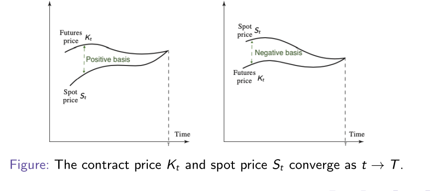
We saw above that the contract price $K$ is usually different to the spot price S of the underlying asset. Our pricing equations, such as

$$K=Se^{(r+s-q)T}$$

for commodity futures, tell us that the difference between $K$ and $S$, which we call the basis, is due to the cost of carry $r + s − q$.

• As the cost of carry changes over time, the basis changes, introducing basis risk: $K$ may not be perfectly correlated with $S$.

The time $t$ basis $B_t$ is the difference between $K_t$ and $S_t$, namely:

Note that the basis approaches 0 over time, and $K_{T}=S_{T}$ at maturity.

6.2 Optimal hedging

Optimal hedging basically means minimising basis risk.

In an imperfect hedging scenario, in which there is basis risk, we choose $h$ that minimises the variance in the liquidation value $L_{t}$.

Then $h$ is called the minimum variance or optimal hedge quantity.

• At time $t = 0$, $A_{t}$ and $K_{t}$ are unknown, thus random variables.

We use the following notation:

• $σ_{A_t}$ is the standard deviation (volatility) in $A_t − A$.
• $σ_{K_t}$ is the standard deviation (volatility) in $K_t − K$.
• $ρ$ is the correlation between $A_t − A$ and $K_t − K$.

We can prove that the optimal or minimum variance hedge quantity $h$, which minimises the variance in the above liquidation value, or equivalently minimises basis risk, is given by

$$h=\rho \frac{\sigma_{A_{t}}Q}{\sigma _{K{t}}m}$$

• we use average historical returns to calculate standard deviations and sample correlation

• Then the optimal hedge quantity is given by

  $$h = \bar{\rho} \frac{\bar{\sigma}_{A}V }{\bar{\sigma}_KF}$$

Where

$$V = AQ \; \; \; \text{and} \;\;\;\; F=Km$$

The CAPM beta β of a share is calculated from historical returns, and is given by

$$\Beta = \bar{\rho} \frac{\bar{\sigma}_A}{\bar{\sigma}_P}$$

Hence β is the optimal hedge ratio and the optimal hedge quantity is

$$h = \Beta \frac{V}{F}$$

where $V = AQ$ is our portfolio value and $F=Km$ is the notional value of 1 contract.