FINM3405 Revision

lecture 4-8 Options

1. Definitions and Concepts

2. Moneyness (ITM, ATM, OTM).

3. Payoffs vs profits (including the premium).

4. Main contracts and markets, contract specifications.

5. Pricing bounds and put-call-parity.

6. American call premium = European call premium when no dividends.

7. Time value and intrinsic value.

8. European option premiums/prices via the Black-Scholes model:

• 8.1. On non-dividend paying assets.
• 8.2. For dividend/income paying assets.
• 8.3. For currencies (simply viewed as dividend paying assets).

9. Black-Scholes assumption of geometric Brownian motion and consequent log-normal distribution of the underlying asset’s price, or normal distribution of the asset’s returns.

10. Simulating geometric Brownian motion in preparation for the Monte Carlo approach to derivative security pricing.

11. Heuristic (non-rigorous) discussion of risk-neutral pricing.

12. Heuristic (hand-waving) interpretation of the factors affecting option prices, and quantification of this via the Black-Scholes model Greeks.

13. Using delta ∆ and gamma Γ to predict small changes in option prices due to small changes in the price of the underlying asset (in preparation for delta and delta-gamma hedging).

14. More detailed discussion of theta θ and associated concept of time decay, and how it relates to moneyness.

15. Scholes Hedging

• 15.1 Static delta hedging
• 15.2 Static delta-gamma hedging
• 15.3 Dynamic delta hedging.

16. Implied volatility

• 16.1 volatility smile and term structure
• 16.2 related VIX index enabling volatility to be directly traded.

17. Trading strategies and their payoff and profit/loss diagrams.

18. Binomial and Monte Carlo numerical option pricing methods:

• 18.1 The need for numerical methods:
• 18.2 Price more complex derivative securities.
• 18.3 More complex pricing methods than the Black-Scholes model, in particular because returns are not normally distributed.

19. 1-period binomial model for European option price and delta.

• 19.1 American Options
• 19.2 Path Dependent Options
• 19.3 European Chooser Options
• 19.4 Lookback Options
  • 19.4.1. Fixed-Strike lookback Options
  • 19.4.2. (European) Floating-Strike Lookback Options
• 19.5 (European) Barrier Options
  • 19.5.1 Knock-in Barrier Options
  • 19.5.2 Knock-out Barrier Options
• 19.6. (European) Asian Options
  • 19.6.1. Fixed-Strike Asian Options
  • 19.6.2. (European) Average-strike Asian options

Aside - Notation

• We work on a given time interval $0 ≤ t ≤ T$ where:
  • Time $t = 0$ is the date we enter into a contract.
  • Time $T$ is the expiry date.
  • Time $t$ is some intermediate date $0 ≤ t ≤ T$.
• $S_t$ is the underlying asset’s price at time $t$.
  • We write $S = S_{0}$ to reduce notation.
• $r$ is the risk free rate.
• $K$ is the strike or exercise price (some authors use X).
• $C_{t}$ and $P_{t}$ are the call and put prices (premiums) at time $t$.
  • Again, we write $C = C_{0}$ and $P = P_{0}$.
• $q$ dividend yield

Black Scholes

• $\sigma$ is the volatility of the underlying asset

1. Definitions and Concepts

Recall that there is two types of plain vanilla European options:

• Call option: Gives the holder the right but not the obligation to buy the underlying asset for the strike price $K$ on the expiry date $T$.
• Put option: Gives the holder the right but not the obligation to sell the underlying asset for the strike price $K$ on the expiry date $T$.

2. Moneyness

At time $t$ an option is:

• In the money if it has positive intrinsic value:
  • $K < S_{t}$ for a call option.
  • $S_{t} < K$ for a put option.
• At the money if $S_{t} = K$ (intrinsic value is 0).
• Out of the money if its intrinsic value is 0 and $S_{t} \ne K$
  • $S_{t} < K$ for a call option.
  • $K < S_{t}$ for a put option.

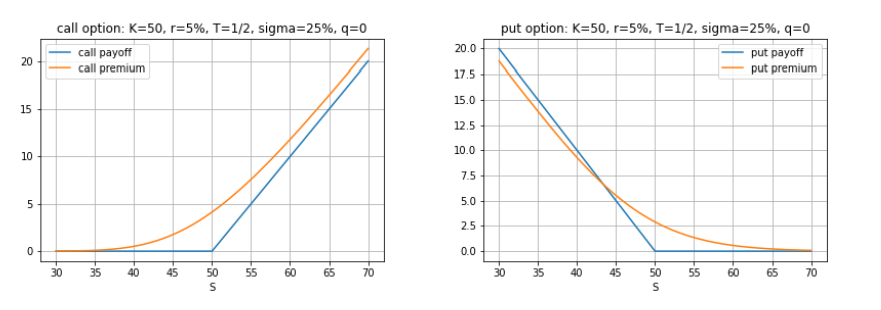
3 Payoffs and Profits

3.1 Payoffs

At any time $t$, an option’s intrinsic or exercise value (IV) is

call $IV_{t} = \max \{ 0, S_{t} − K \}$

and put $IV_{t} = \max \{ 0, K − S_{t} \}$

3.2 Profits

• call holder profit = $\max \{ 0, S_T − K \} − C$,
• put holder profit = $\max \{ 0, K − S_T \} − P$

and the writer’s (short position) profits are the negative of these:

• call writer profit = $C − \max \{ 0, S_T − K \}$,
• put writer profit = $P − \max \{ 0, K − S_T \}$.

4. Main contracts and markets, contract specifications.

• Will be given in final assignment

5. Pricing bounds and put-call parity

5.1 put-call parity

Developing mathematical models for pricing options (calculating the fair value of the option premium), such as the Black-Scholes option pricing model, is a major part of the theory and practice of options.

Form a portfolio long 1 European call and short 1 European put, both with the same underlying, strike and expiry.

This portfolio’s current price is C − P and its payoff at expiry is

$$\text{portfolio payoff} = \underbrace{\max\{0, S_T - K\}}_{\text{long call}} - \underbrace{\max\{0, K - S_T\}}_{\text{short put}}$$

5.2 Pricing bounds

1. First note that American options are worth at least as much as European options over the same underlying asset and with the same strike and expiry:

$$0 \le C_{Eu} \le C_{Am}$$

and

$$0 \le P_{Eu} \le P_{Am}$$

American options can be exercised any time up to and including expiry

5.2.1 Option Pricing Bounds - American

Lower Pricing bounds - American 2. American options are worth at least their intrinsic (exercise) value:

$$\max \{0, S − K \} ≤ C_{Am}$$

and

$$\max \{0, K − S \} ≤ P_{Am}$$

because they can be exercised immediately

Upper Pricing bounds - American 3. American calls can never be worth more than the underlying spot price, and American puts can never be worth more than the strike:

$$C_{Am} ≤ S$$

and

$$P_{Am} ≤ K$$

Combined

Combining the lower and upper bounds from the previous two slides leads to the important pricing bounds for American options:

$$\max \{ 0, S − K \} ≤ C^{Am} ≤ S$$

And

$$\max \{ 0, K − S \} ≤ P^{Am} ≤ K$$

5.2.2 Option Pricing Bounds - European

Upper Pricing bounds - European

$$0 \le P^{Eu} \le Ke^{-rT}$$

because a European put can only be exercised at expiry, where it is known with certainty that their maximum payoff at expiry is $K$.

From this, deep in-the-money European puts can have negative time value (their premium can be less than their intrinsic value).

Combined

European calls

$$\max \{ 0, e^{-qT}S-e^{-rT}K \} \le C^{Eu} \le S$$

European puts

$$\max(0, e^{-rT}K - e^{-qT}S) \le P^{Eu} \le Ke^{-rT}$$

• Key note: discount exercise price to $t_0$

6. No early exercise of American calls

early exercise is never optimal for an American call option on a non-dividend-paying stock

• Under no dividends, so $q = 0$, from above we start with

$$\max (0, S − e^{−rT}K) ≤ C^{Eu} ≤ C^{Am}$$

• If $r > 0$ then $e^{−rT} K < K$ and we get a strict inequality

$$\max(0, S − K) < \max (0, S − e^{−rT}K) ≤ C^{-rT} ≤ C^{Am}$$

But $\max(0, S − K)$ is just the call’s intrinsic value. So if there’s no dividends, call options will always have strictly positive time value.

7. Time value and intrinsic value.

From above, we noticed that call options on non-dividend-paying stocks have a premium that is strictly larger than the option’s intrinsic value.

$$\text{time value = premium − intrinsic value}$$

8. European option premiums/prices via the Black-Scholes model

The Black-Scholes European option pricing model is a mathematical equation for pricing plain vanilla European call and put options.

8.1 European option premiums on non-dividend paying assets

Black-Scholes European call option pricing model is

$$C = S\mathcal{N} (d_{1}) − Ke^{−rT}\mathcal{N} (d_{2})$$

Where:

$$d_{1} = \frac{\log \frac{S}{K} + (r+\frac{1}{2}\sigma ^{2})T}{\sigma \sqrt{T}}$$

And

$$d_{2} = d_{1} - \sigma \sqrt{T}$$

$$= \frac{\log \frac{S}{K} + (r -\frac{1}{2}\sigma ^{2})T}{\sigma \sqrt{T}}$$

8.2 European option premiums incorporating dividends

pricing equations for European call $C$ and put #$P$ options become

$$C = Se^{-qT}\mathcal{N} (d_{1}) − Ke^{−rT}\mathcal{N} (d_{2})$$

$$P = Ke^{−rT}\mathcal{N} (-d_{2}) - Se^{-qT}\mathcal{N} (-d_{1})$$

Where:

$$d_{1} = \frac{\log \frac{S}{K} + (r - q + \frac{1}{2}\sigma ^{2})T}{\sigma \sqrt{T}}$$

And

$$d_{2} = d_{1} - \sigma \sqrt{T}$$

$$d_{2} = \frac{\log \frac{S}{K} + (r - q - \frac{1}{2}\sigma ^{2})T}{\sigma \sqrt{T}}$$

8.3. European option premiums for currencies

We view the foreign risk-free rate $r_f$ as the “dividend” on the underlying asset (the foreign currency):

$$C_{f:d} = S_{f:d}e^{-r_fT}\mathcal{N} (d_{1}) − K_{f:d}e^{−r_dT}\mathcal{N} (d_{2})$$

$$P_{f:d} = K_{f:d}e^{−r_dT}\mathcal{N} (-d_{2}) - S_{f:d} e^{-r_fT}\mathcal{N} (-d_{1})$$

Where:

$$d_{1} = \frac{\log \frac{S_{f:d}}{K_{f:d}} + (r_d - r_f + \frac{1}{2}\sigma ^{2})T}{\sigma \sqrt{T}}$$

and

$$d_{2} = d_{1} - \sigma \sqrt{T}$$

$$= \frac{\log \frac{S_{f:d}}{K_{f:d}} + (r_d - r_f - \frac{1}{2}\sigma ^{2})T}{\sigma \sqrt{T}}$$

9. key features/Assumptions of Black Scholes

1. We’re using historical volatility for σ but in practice options traders tend to use the Black-Scholes model with “rules of thumb” and their own estimates of σ.
2. Our dividend yield may not be accurate: We assumed a continuously compounded yield. It should be a forecast. And should we incorporate dividend imputation/franking?

Geometric Brownian Motion

• underlying assets follows geometric brownian motion
• Stock price $S_t$ in black Scholes model is log-normally distributed

10. Simulating geometric Brownian

• You can iteratively simulate geometric brownian motion over each subinterval to create a complete path
• Used in the Monte-Carlo simulation pricing of options (outlined below)

So in the risk-neutral pricing approach the value of a European option is

• the present value of its expected future payoff
• but discounted at the risk-free rate r.

12. Factors affecting options prices

How each of the input variables $K$, $S$, $r$, $T$, $σ$ and $q$ impact option premiums

We’re interested in the sensitivity of option prices to the other variables $S$, $r$, $T$ and $σ$, and we give these sensitivities special Greek names:

• Delta ∆ is the sensitivity of the option price to S.
• Gamma Γ is another measure of the relation between prices and S.
• Rho ρ is the sensitivity of the option price to rates r.
• Vega ν is the sensitivity of the option price to volatility σ.
• Theta θ is the sensitivity of the option price to time T.

12.1 Delta and Gamma

We know that as $S$ increases, calls premiums rise and put premiums fall.

We quantify this mathematically with the delta ∆, given by

$$∆_{C} = N(d_{1}) \: \: \text{and} \: \: ∆_{P} = N(d_{1}) − 1$$

Importantly, note the following

$$0 < ∆_{C} < 1 \: \: \text{and} \: \: -1 < ∆_{P} < 0$$

We interpret ∆ as the change in the premium due to a change in S, giving us the approximations

$$dC \approx \Delta _{c} dS \: \: \text{and} \: \: dP \approx \Delta _{p} dS$$

where $dC$ and $dP$ are a change in the premium and $dS$ a change in $S$.

We calculate the “new” premiums due to a change in S as

$$C_{new} \approx C + dC \: \: \text{and} \: \: P_{new} \approx P+dP$$

12.2 Rho

Rho ρ is the change in the premium from a change in $r$, and is given by

$$\rho_c = KTe^{-rT}\mathcal{N}(d_2)$$

and

$$\rho_p = KTe^{-rT} \left[ \mathcal{N}(d_2) -1 \right]$$

Where

$$0 < \rho_c$$

and

$$\rho_p < 0$$

Example for call prices:
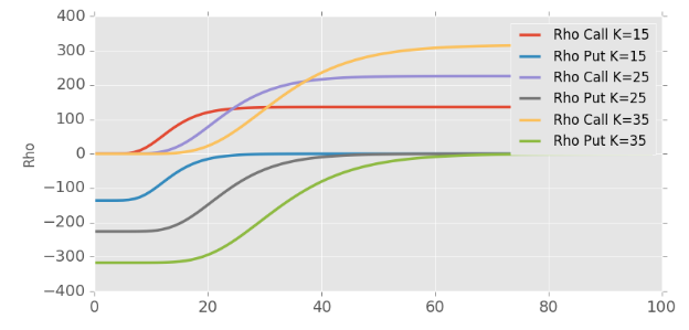(x axis is underlying stock price)

As $r$ increases, call premiums increase but put premiums decrease.

• An intuitive explanation for this is the present value $e^{−rT}K$ of the strike that the holder pays in a call, or receives in a put, decreases.

12.3 Vega

Vega ν is the change in the premium from a change in σ, and is given by:

$$\nu = Sf(d_{1})\sqrt{T}$$

• Same for calls and puts

with $f(x)$ the PDF of a standard normal random variable. Note that

$$0 < \nu$$

As σ increases, option premiums increase.

12.4 Theta

Theta θ is a bit ambiguous. It gives the negative of the change in the premium from a change in $T$. And the equations are more complex:

$$\theta_c = -\frac{Sf(d_1)\sigma}{2\sqrt{T}} -rKe^{-rT}\mathcal{N}(d_2)$$

and

$$\theta _p = \theta _c + rKe^{-rT}$$

θ is the negative of the partial derivative of the premium with respect to T, telling us the impact of approaching expiry.

$$\theta _c < 0$$

but we may have

$$\theta _p \le 0$$

and

$$0 \le \theta _p$$

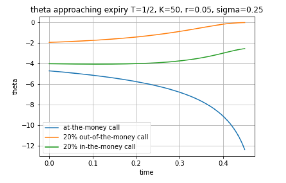
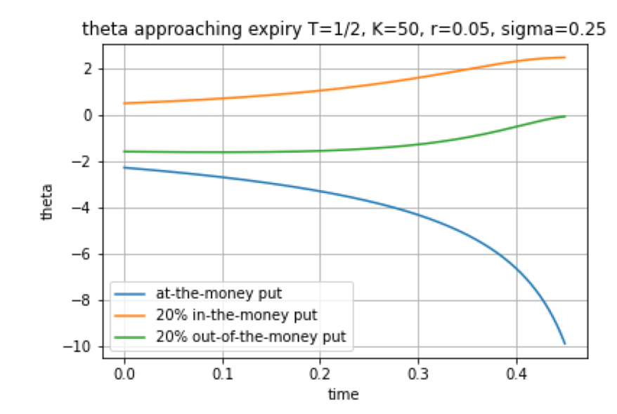
• Impact of time on puts is ambiguous: From $\theta _{P} = \theta _{C} + rKe^{-rT}$ deep in-the-money put (large K) premiums may increase as expiry nears.
• This relates to something said last week: A deep in-the-money put is already close to its maximum payoff of K, so not much more payoff can be realised at expiry, but there is still a chance of an unfavourable movement in the asset price. But as we approach expiry, there is less chance of an unfavourable movement.

12.4.1 Time Decay

Premiums usually fall as expiry approaches

• Time decay works for option writers and against option holders.
• θ is most negative for options close to at-the-money.
• θ in fact gets more negative for options close to at-the-money as expiry approaches: Time decay “speeds up” as expiry approaches.

Theta Call	Theta Put

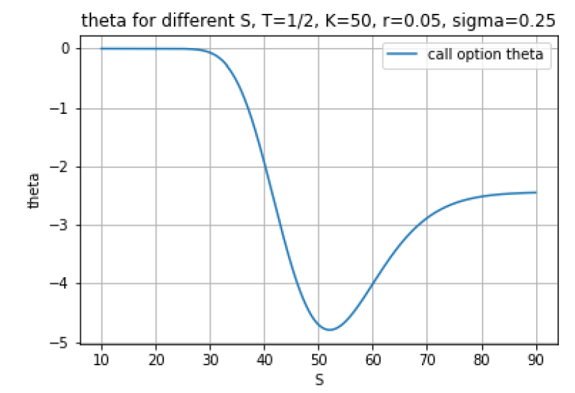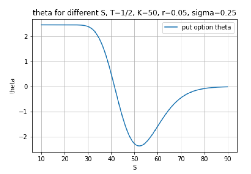13. Scholes Hedging

13.1 Static Delta Hedging

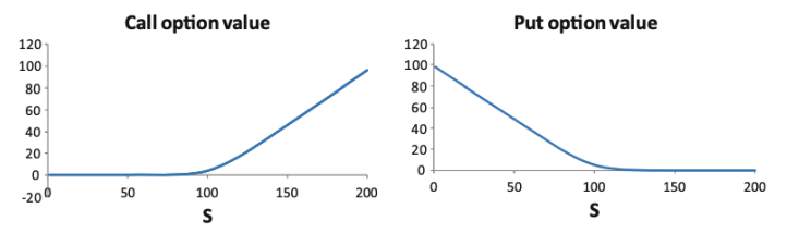
Recall the basic long call and put option payoff and premium plots:

Delta hedging involves taking a position in the asset to hedge an option position against small movements in the asset’s price.

An option’s delta is an approximation of the change in the premium due to a change dS in the price S of the underlying asset:

$$dC ≈ ∆_C dS \; \; \text{and} \; \; dP ≈ ∆_P dS.$$

Static delta hedging with h options

The value of a portfolio of $h$ calls and $Q$ units in the underlying asset is

$$V = QS + hC$$

The value of a portfolio of $h$ puts and $Q$ assets is $V = QS + hP$. Its change is $dV ≈ (Q + h∆_P )dS$ so we set

$$Q = −h∆_P$$

or

$$Q = −h∆_C$$

for hedging options

13.2 Delta-Gamma hedging

We can use delta-gamma hedging to improve the delta hedging of an option position by taking a position in the asset and a different option.

For delta-gamma hedging we calculate how many units $Q$ in the asset and $k$ in another option we need in order to hedge against small changes $d$S in the price $S$ of the underlying asset.

The value of a portfolio of $Q$ units in the asset, $h$ units of one option, and $k$ units of another, different option is given by

$$V = QS + hV_1 + kV_2$$

where $V_1$ and $V_2$ are the respective option premiums.

We can show that the solution is

$$Q = -h \frac{\Delta _1 \Gamma _2 - \Delta _2 \Gamma _1}{\Gamma _2}$$

And

$$k = \frac{Q \Gamma _1}{\Delta _1 \Gamma _2 - \Delta _2 \Gamma _1}$$

IMPORTANT:

• $h$ is related to the first option (and $\delta_1$ and $\gamma_1$)
• $k$ is related to the second option ($\delta_2$ and $\gamma_2$)

13.3 Dynamic delta hedging

• Not examined in final exam

14. Implied Volatility

In the Black-Scholes European option the only unobservable parameter is the volatility σ.

Given observed option prices $C$ or $P$ and observable market variables $S$, $K$, $r$ and $T$, an option’s implied volatility is the volatility parameter σ that yields Black-Scholes prices equal to $C$ or $P$.

We have to code numerical (iterative) techniques on computers.

In markets, Black-Scholes implied vols are not constant but display:

• A volatility smile or smirk over the range of strike prices.
• A volatility term structure over the range of expiry dates.

Volatility smirk/smiles

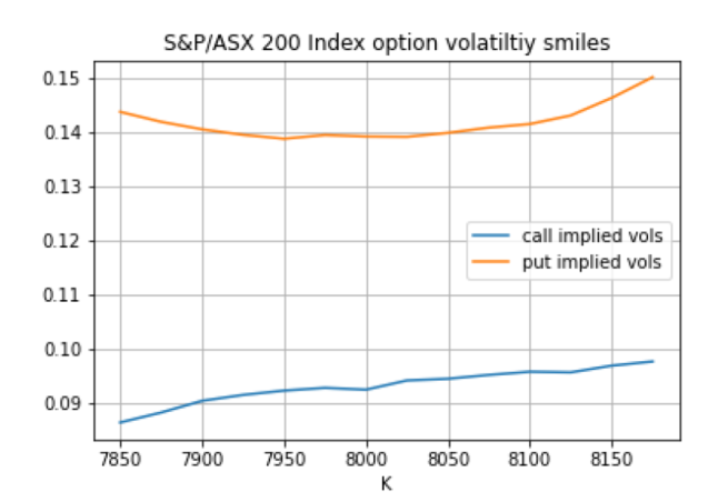Remark We see this from the volatility smile and term structure:

• The volatility parameter σ we need to use to get the Black-Scholes model to match observed option premiums is not constant across the range of strike prices and expiries

Consequently traders use:

• Rules of thumb, intuition and market conventions and experience to determine the σ parameter to use in the Black-Scholes model.
• Other, more complex and accurate option pricing models.

14.1 VIX index

• The Cboe VIX Index measures “market wide” implied vols:

It “is a calculation designed to produce a measure of constant, 30-day expected volatility of the U.S. stock market, derived from real-time, mid-quote prices of S&P 500 Index (SPX) call and put options.”

VIX index example

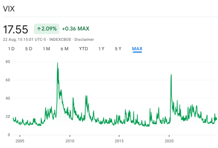A value of 17.55 means that average implied vols of 30 day S&P 500 Index options, thus the market’s 30 day volatility expectations, is 17.55%.

15 Trading Strategies

1. Directional strategies: Speculate on the direction of the price of the underlying asset, similar to taking calls and puts.
2. Volatility strategies: Speculate on high or low asset volatility, or changes in implied vols, often incorporating delta neutrality.
3. Time: Strategies that seek to take advantage of time decay, typically assuming low asset volatility and relatively constant implied vols.

15.1 Directional strategies

Directional strategies seek to speculate on a directional change in the price of the asset, but at a lower upfront cost to the basic strategies of taking calls and puts, while still maintaining limited downside risk.

15.1.1 Bull Spread

Suppose we want to speculate on an increase in the asset price:

We could take an ATM call with strike $K = 50$, costing $C_1 = 4.13$. But also write an OTM call with strike $K_2 = 55$.

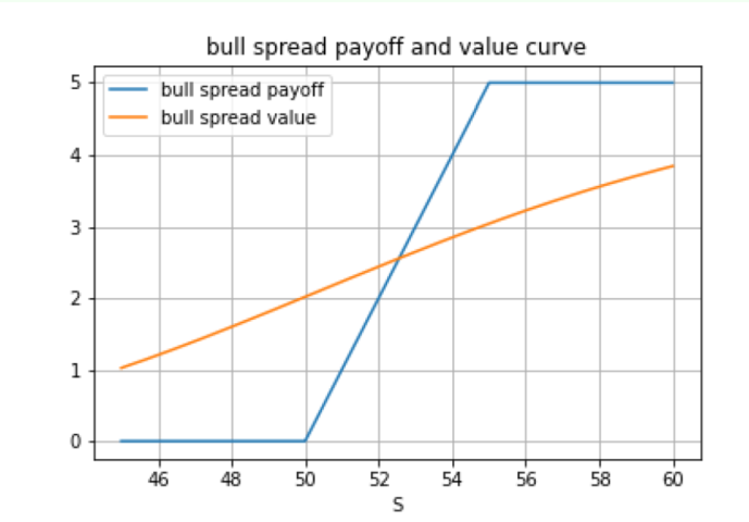
A bull spread has lower downside risk and “profits sooner” compared to the basic long call, but its upside profits are capped.

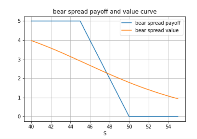
15.1.2 Bear Spread

Speculate on a decrease in the asset price:

We can lower the cost of taking a put with strike $K = 50$ by also writing a put with strike $K_2 = 45$.

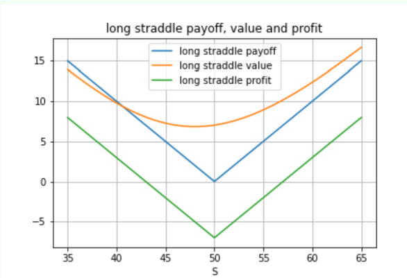
15.2 Volatility Strategies

15.2.1 Long Straddle

Suppose we think that the asset price will be volatile:

We could take ATM calls and puts both with strike K = 50, a strategy called a long straddle with payoff and profit:

15.2.2 Short Butterfly

As shown above

15.2.3 Short Straddle

Suppose that we expect a period of low volatility

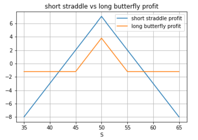
15.2.4 Long Butterfly

As shown above

16. Binomial and Monte Carlo numerical option pricing methods

16.1 & 16.3 Rationale

1. When applying the Black-Scholes framework to derive pricing models for more complex, exotic derivatives (even just for American options), we immediately run into the scenario of being unable to derive closed-form, analytical solution equations.
2. We may also want to apply more complex derivative security pricing frameworks than the Black-Scholes framework (say the Heston stochastic volatility, or the Merton jump-diffusion, frameworks), but again we immediately run into the same problem.

Stylised features of financial returns:

• Non-normality:
  • Spiked mean.
  • Narrow shoulders.
  • Fat tails.
  • Skewness, or at least extreme negative return events.
• Volatility clustering or regimes (non-constant volatility).

16.2 Methods

1. Lattice type methods like the binomial and trinomial models.
2. Monte Carlo methods:

• Motivated by the risk-neutral approach to derivative security pricing.

3. Partial differential equation numerical solution methods:

• Motivated by the partial differential equation (PDE) approach to derivative security pricing (we avoid it in FINM3405).

17. Binomial model for European option price and delta

17.1 1-Period

• One trading period of length $T$ years to the option’s expiry.
• Starting at S, two possible outcomes for the underlying asset:
  1. Up to $S_u = Su$, where $u$ is the asset’s up factor.
  2. Down to $S_d = Sd$, where $d$ is the asset’s down factor.
• A risk-free rate $r$ satisfying $d < e^{rT} < u$.

The call option’s payoffs in each possible outcome of the price of the underlying asset are:

$C_u = \max(0, S_u − K)$

$C_d = \max(0, S_d − K)$

Call option

$$C = e^{-rT}[qC_u + (1-q)C_d]$$

Where

$$q = \frac{e^{rT} - d}{u-d}$$

17.1.1. Up and down factors

1. The Jarrow-Rudd (JR) scheme derives

$$u=e^{(r - \sigma^2 /2)T + \sigma \sqrt{T}} \;\;\; \text{and} \;\;\; d = e^{(r - \sigma ^2 / 2) T - \sigma \sqrt{T}}$$

17.2 Multi-period

For the multi-period binomial model we simply:

1. Discretise the interval [0, T] into N + 1 equally-spaced dates ${t_0 , t_1 , . . . , t_N }$ with $t_0 = 0, t_N = T$ and spacing $dt = T/N$.
2. Build an asset price tree starting at $S$ as per the next slide.
3. Calculate the option premium by recursively stepping backwards in time in the tree and using the 1-period pricing formula each step.

Build asset price tree of S

To build the asset price tree, we note that the asset price can go up by a factor of $u$ or down by a factor of $d$ at each time step.

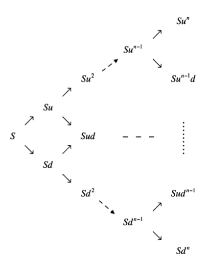
Asset price S$_{iN}$ took $i$ up steps and thus $N − i$ down steps.

• At time step $j$ there is $j + 1$ asset prices $S_{ij} = Su^i d^{j−i}$ for $i = 0, 1, . . . , j$. Asset price $S_{ij}$ took $i$ up steps and thus $j − i$ down steps.

Calculate Asset Price tree of C/P:

We calculate call prices as follows:

• The call option payoff s at expiry (time T) are

$$C_{iN} = \max \{0, S_{iN} − K \}$$

for $i = 0, 1, . . . , N$.

• We let $C_ij$ denote the call price at time step $j$ when the underlying asset took $i$ up steps (and thus $j − i$ down steps)

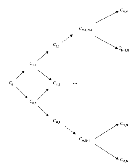
• From the previous iteration in the recursion, we know the call prices $C_{i+1,j+1}$ (up step) and $C_{i,j+1}$ (down step) at time step $j + 1$.
• We calculate $C_{ij}$ as follows:

$$C_{ij} = e^{-rdt}\left[ qC_{i+1, j+1} + (1-q)C_{i, j+1}\right]$$

17.3 Binal price deltas

$$\Delta = \frac{C_u - C_d}{S(u-d)}$$

$$\Delta = \frac{P_u - P_d}{S(u-d)}$$

17.3 Rationale of Risk-neutral approach

-- to complete

18. Monte Carlo Pricing of European Options

Option prices are given by

$$C = e^{-rT} \mathbb{E} \left[ \max \{ 0, S_T - K \} \right]$$

and

$$P = e^{-rT} \mathbb{E} \left[ \max \{ 0, K - S_T \} \right]$$

Where $S_T$ is log-normally distributed as per geometric Brownian motion.

To price options via the Monte Carlo method we:

• Simulate $N$ sample paths of geometric Brownian motion of length $M + 1$ as per next slide to get $N$ asset prices $S_{iM}$ for $i = 1, . . . , N$

19. Pricing American and path dependent options

19.1 American Options (using Binomial Tree)

An American option gives the holder the right (but not the obligation) to exercise it at any point up to and including the expiry date $T$.

American options are worth at least as much as European options:

$$0 ≤ C_{Eu} ≤ C_{Am}$$

and

$$0 ≤ P_{Eu} ≤ P_{Am}$$

American options are worth at least as much as their intrinsic value:

$$\max{0, S − K} ≤ C_{Am}$$

and

$$\max{0, K − S} ≤ P_{Am}$$

The adjustment to price American options is:

A each node, set the American option price equal to the maximum of the “1-step European price” and the option’s intrinsic value:

The (American and European) option payoffs at expiry are

$$C^{Am}_{iN} = \max \{ 0, S_{iN} - K \}$$

and

$$P^{Am}_{iN} = \max \{ 0, K - S_{iN} \}$$

The “1-step European” option prices at node ij on the tree are

$$C^{Eu}_{ij} = e^{-rdt}\left[ qC^{Am}_{i+1, j+1} + (1-q)C_{i, j+1}^{Am} \right]$$

$$P^{Eu}_{ij} = e^{-rdt}\left[ qP^{Am}_{i+1, j+1} + (1-q)P_{i, j+1}^{Am} \right]$$

Hence, the American option prices at node $ij$ are

$$C^{iv}_{ij} = \max \{C^{Eu}_{ij}, C^{iv}_{ij} \}$$

$$P^{iv}_{ij} = \max \{P^{Eu}_{ij}, P^{iv}_{ij} \}$$

19.2 Path Dependent Options

A European option is path dependent if its payoff is calculated from the underlying asset’s path travelled over the option’s life.

19.3 European Chooser Option (binomial method)

A European chooser option is similar to a plain vanilla European option except that it allows the holder to choose at some date $t$ choose (the choice date) over the option’s life if the option is a call or a put

• The choice date satisfies $0 < t_{\text{choose}} < T$.

Modification to original Binomial Tree

• When working backwards recursively through the binomial tree to calculate the European call and put option prices, on each node of the choice date select the chooser option’s value as the maximum of the call and put values. From there work backwards recursively as per normal for the chooser option, ignoring the call and put

19.4 Lookback options (Monte-Carlo)

A lookback option’s payoff at expiry depends on the maximum or minimum prices of the underlying asset over the life of the option

19.4.1 Fixed-Strike lookback Options

European fixed-strike lookback options are very similar to plain vanilla European options except the “final price” of the underlying asset used in calculating the payoff is not the asset price $S_{T}$ but instead the maximum $S_{max}$ or minimum $S_{min}$ asset price reached over the option’s life:

The maximum and minimum asset prices of path $i$ are given by

$$S_{i, max} = \underbrace{\max}_{j=0,...,M}S_{ij}$$

$$S_{i, min} = \underbrace{\min}_{j=0,...,M}S_{ij}$$

• call payoff = $\max \{ 0, S_{max} − K \}$
• put payoff = $\max \{ 0, K - S_{min} \}$

The Monte Carlo Option prices are then simply

$$C = e^{-rT} \frac{1}{N} \sum ^N _{i=1} \max \{ 0, S_{i, \max } - K \}$$

$$P = e^{-rT} \frac{1}{N} \sum ^N _{i=1} \max \{ 0, K - S_{i, \min } \}$$

19.4.2. (European) Floating-Strike Lookback Options

European floating-strike lookback options differ from fixed-strike options by instead setting the strike price $K$ to be the maximum $S_{max}$ or minimum $S_{min}$ asset prices over the life of the option. Their payoffs are

$$\text{call payoff} = \max \{ 0, S_T - S_{\min } \}$$

$$\text{put payoff} = \max \{ 0, S_{\max } - S_T\}$$

So, after calculating the N asset price paths $\{ S_{i0} , S_{i1} , . . . , S_{iM} \}$ for i = 1, . . . , N by simulating geometric Brownian motion, and calculating the minimum S i,min and maximum S i,max prices for each path, the Monte Carlo floating-strike lookback option prices are then simply

$$C = e^{-rT} \frac{1}{N} \sum ^N _{i=1} \max \{ 0, S_{iM} - S_{i, \min } \}$$

$$P = e^{-rT} \frac{1}{N} \sum ^N _{i=1} \max \{ 0, S_{i, \max } - S_{iM} \}$$

19.5 (European) Barrier Options

They are effectively plain vanilla European options whose payoff's “knock in” or “knock-out” if the price of the underlying asset hits a barrier $B$ at some point over the life of the option:

19.5.1 Knock-in Barrier Options

European knock-in options are activated if the price of the underlying asset hits the barrier B at some point of the option’s life.

The payoffs are then the usual

• $\max \{ 0, S_T − K \}$ for a call
• $\max \{ 0, K − S_T \}$ for a put

If the barrier is never hit, the option is never activated and expires worthless

There’s two kinds of knock-in options depending on the relation between $B$ and $S$

1. Up-and-in options set $B > S$, noting that typically $K ≈ S$.
2. Down-and-in options set $B < S$, noting that typically $K ≈ S$.

The Monte Carlo pricing of knock-in options is a simple modification to the above, simply to check each path to see if the barrier was hit.

• If the barrier is not hit, the value of the simulation is $0$

19.5.2. Knock-out Barrier Options

European knock-out options are deactivated if the price of the underlying asset hits the barrier B at some point of the option’s life.

If the barrier is never hit, the option stays alive and the payoff's are the usual $\max \{ 0, S_T − K \}$ for a call and $\max \{ 0, K − S_T \}$ for a put. There’s two kinds of knock-outs depending on the relation between B and S:

1. Up-and-out options set $B > S$, noting that typically $K ≈ S$.
2. Down-and-out options set $B < S$, noting that typically $K ≈ S$.

The Monte Carlo pricing of knock-out options is a simple modification to the above for knock-in options, namely a reversal of the logical conditions on the payoffs if the barrier was hit.

19.6. (European) Asian Options

A European Asian or average option’s payoffs depend on the average underlying asset price $\bar{S}$ over the life of the option.

There’s two general types of Asian options:

1. Fixed-strike Asian options.
2. Average-strike Asian options.

19.6.1. Fixed-Strike Asian Options

European fixed-strike Asian options are very similar to plain vanilla European options except the “final price” of the underlying asset used in calculating an option’s payoff is not the asset price itself but the average asset price $\bar{S}$ over the life of the option. Their payoffs are

It is simple to use Monte Carlo simulation to price them:

So, after calculating the $N$ asset price paths $\{ S_{i0} , S_{i1} , . . . , S_{iM} \}$ for $i = 1, . . . , N$ by simulating geometric Brownian motion, the average price of path $i$ is

$$\bar{S}_{i} = \frac{1}{M} \sum^{M}_{j=0}S_{ij}$$

(arithmetic average). The payoffs for path $i$ are

• call payoff = $\max \{ 0, \bar{S}_{i} − K \}$
• put payoff = $\max \{ 0, K - \bar{S}_{i} \}$

Put and call prices are then:

$$C = e^{-rT} \frac{1}{N} \sum ^N _{i=1} \max \{ 0, \bar{S}_{i} − K \}$$

$$P = e^{-rT} \frac{1}{N} \sum ^N _{i=1} \max \{ 0, K - \bar{S}_{i} \}$$

19.6.2. Average-strike Asian options

European average-strike Asian options differ from fixed-strike Asian options by instead setting the strike price $K = \bar{S}$ to be the average asset price $\bar{S}$ over the life of the option. So, their payoff s are simply

• call payoff = $\max \{ 0, S_T − \bar{S} \}$
• put payoff = $\max \{ 0, \bar{S} - S_T \}$