FINM3405 Revision

Value at Risk (VaR) and Expected Shortfall (ES)

1. Basic concepts relating to risk, including:

• Types: market, default, liquidity, operational.
• Portfolio expected return and standard deviation (volatility).
• Concepts related to the normal distribution in preparation for calculating value at risk (VaR) and expected shortfall (ES).
• The need for simple, single measures of market risk like VaR and ES.
• VaR and ES definitions, basic concepts, and differences.
• Potential shortcoming of VaR and consequent need for ES.
• Calculating VaR and ES via 2 methods:
  • Parametric approach assuming normally distributed returns.
  • Nonparametric approach directly using historical data.
• Parametric portfolio VaR, worst case VaR, diversification benefits.

1. Definitions and Concepts

1.1 Risk Types

We could classify risk into the following 4 broad categories:

1. Market risks: These are the risks we’ve mostly been discussing this semester, namely risks due to movements in market variables such as interest rates, exchange rates, stock prices, commodity prices, etc.
2. Liquidity risk: The inability to sell or liquidate assets and financial securities quickly and at prices close to fair market values.
3. Credit risk: The risk of loss due to borrowers and counterparties failing to meet, and thus defaulting on, their payment obligations.
4. Operational risks: “All others” including human error, fraud and theft, model risk, technology failure, legal risk, weather events, etc.

1.2 Individual security risk

• Let $\{R_1 , . . . , R_N\}$ be $N$ time period returns for a financial asset.

Recall that the mean return is given by

$$\mu = \frac{1}{N} \sum ^N _{i=1} R_i$$

volatility in returns is

$$\sigma = \sqrt{\sum ^N _{i=1} \frac{(R_i - \mu)^2}{N-1}}$$

1.3 Portfolio risk and return

Portfolio mean return is

$$µ = w_1 µ_1 + w_2 µ_2$$

Portfolio standard deviation in returns is:

$$\sigma_p = \sqrt{w^2_1\sigma^2_1 + w^2_2\sigma^2_2 + 2w_1w_2\sigma_{1,2}}$$

2. Normal distribution

• Assume returns are normally distributed
  • mean $\mu$ and variance $\sigma ^2$ completely characterise the probability distributed of the returns

The CDF of the standard normal distribution ($\mu = 0$ and $\sigma^2=1$) is

$$\mathcal{N}(z) = \mathbb{P}(r \le z) = \frac{1}{\sqrt{2 \pi}} \int ^z _{-\infty} e^{-\frac{x^2}{2}}dx$$

For negative z-values, it gives the following “left tail” area or probability:

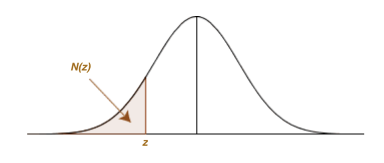
When doing VaR and ES calculations, we’re interested in the following “left tail” areas α = N (z) and z-values z that give them:

• $α = N (−1.645) = 0.05.$
• $α = N (−1.96) = 0.025.$
• $α = N (−2.326) = 0.01.$

To find the z-value $z_α$ corresponding to a given left tail probability or area $\alpha$ for a normal distribution with mean µ and variance $\sigma^2$ we set

$$z_α = µ + zσ$$

where $z$ is the z-value for a standard normal distribution corresponding to the left tail probability $α = N(z)$

3. Var and ES definitions

Using tail probability $α = 1 − p$, value at risk (VaR) answers:

What is the maximum dollar loss $VaR_α$ that would be incurred over a given time period with probability p?

2 perspectives:

1. “We will lose at most $VaR α over the time period in p% of cases.”
2. “We will lose at least $VaR α over the time period in α% of cases.”

• VaR α is the value at risk (what we risk losing).
  • It’s the most we’d lose with probability $p = 1 − α$
  • Or the least we’d lose with probability $α = 1 − p$.
• $p$ is the level of confidence.
  • It’s typically set to p = 95%, or p = 97.5%, or p = 99%.
• $α = 1 − p$ is called the tail probability.
  • It’s typically small at α = 5%, α = 2.5%, α = 1%, etc.
• Also, the time period is usually “small” at 1 or 10 days.

$VaR_α$ is possibly best conceptualised graphically:

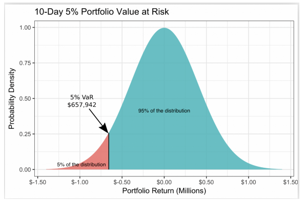
The α = 5% VaR is VaR 0.05 = $657, 942, which in words is:

• VaR 0.05 is the worst outcome over 10 days with p = 95% confidence.
• Or, α = 5% of the time we lose at least VaR 0.05 dollars over 10 days.

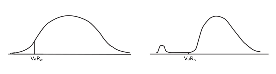
4. Shortcomings of VaR

$VaR_α$ tells us the least amount we expect to lose with tail probability α% in a given time period.

So VaR has the shortcoming that it does not tell us what our expected tail risk or loss or shortfall (ES) is, that is, how much we expect to lose if our portfolio outcomes fall in the α% left tail area of the distribution.

Probabilistically, $ES_α$ is the expected value or mean in the case that our outcomes are worse than (left of) $VaR_α$ for a given tail probability α:

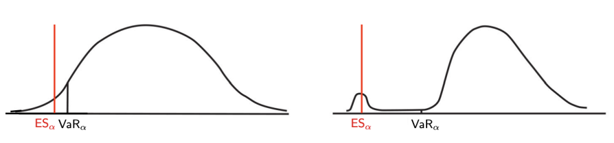
5. Calculating ES:

We cover two contrasting approaches to VaR α and ES α calculation:

1. Parametric: Assumes the distribution of changes dV in our portfolio value V can be described or modelled by a known “parametric family” of probability distributions.

• We assume the normal distribution.
• Uses historical data to estimate the parameters µ and $σ^2$ of the best fitting normal distribution to calculate $VaR_α$ and $ES_α$.

1. Nonparametric: We don’t assume a “parametric family”, but instead use historical data directly to construct histograms and “rank” or “order” or manually “sort” the changes dV in our portfolio value V in order to calculate VaR α and ES α for a given α.

5.1. ES parametric approach

When asset returns are normally distributed with mean $µ$ and variance $σ^2$, for a given left tail probability α we already know that the value at risk $VaR_α$ of the change dV in the portfolio value V is given by

$$VaR_α = −(µ_{dV} + zσ_{dV} )$$

with z the z-value of the standard normal distribution corresponding to the left tail probability $α = N (z)$. The expected shortfall $ES_α$ is

$$\text{ES}_\alpha = -\mu_{dV} + \frac{\sigma_{dV}}{\alpha}f(z)$$

where

$$f(z) = \frac{1}{\sqrt{2\pi}} e^{\frac{-z^2}{2}}$$

f(z) is the standard normal PDF

NOTE:

• in the textbook $X$ is the confidence interval - the formula sheet uses $1-X = \alpha$ for the ES formula

5.1.1 VaR Portfolio

We now want to write the portfolio VaR α in terms of the values at risk $VaR_{α,1}$ and $VaR_{α,2}$ of asset 1 and 2 in the portfolio:

The result we want to remember is the portfolio $VaR_α$ is given by

$$VaR_\alpha = \sqrt{VaR^2_{\alpha , 1}+VaR^2_{\alpha , 2}+2\rho VaR^2_{\alpha , 1} VaR^2_{\alpha , 2}}$$

5.1.2. Diversification benefits

The worst case portfolio $VaR_α$ is thus defined as

$$worst case VaR_α = VaR_{α,1} + VaR_{α,2}$$

So the worst case portfolio $VaR_α$ is when the assets are perfectly correlated (ρ = 1), and is just the sum of the individual VaRs.

We define the benefits from diversification to be

$$\text{diversification benefits} = \text{worst case }VaR_\alpha - VaR_\alpha$$

$$= VaR_{\alpha , 1} + VaR_{\alpha , 2} - VaR_\alpha$$