Lecture 6 - Real Estate Financial Modelling
Objectives
- Know when and how to use discounting and compounding calculations to assess the financial performance of real estate assets
- Be able to prepare a basic DCF model for real estate assets that derives NPV & IRR
- Understand the application of the DCF model in analysing the financial performance of real estate assets and challenges associated with this model
- When to use them and how you use them to assess financial assets
Financial Modelling Mathematics
| Application | Type | Compounding | Discounting |
|---|---|---|---|
| FV of $1 | Capital sum | ||
| PV of $1 | Capital sum | Reciprocal of FV of $1 | or |
| FV of $1pp | Cash flow | ||
| Sinking Fund Factor | Cash flow | Reciprocal of FV of $1pp | |
| PV of $1pp | Cash Flow | ||
| Mortgage Factor | Cash Flow |
Compounding vs discounting
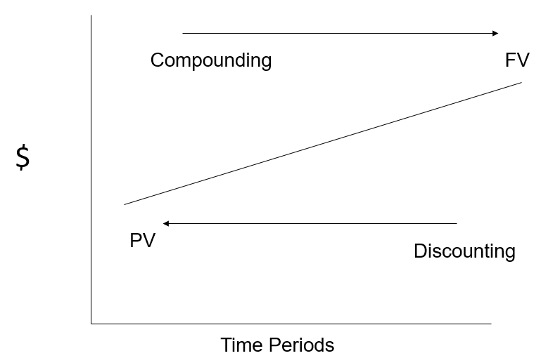
1) The future value of $1 (FV)
Definition: The amount to which $1 will grow at a given rate of interest for a given period of time.
- This is derived using the basic compound interest formula
- The formula will provide a factor for the compounding of one unit (or $1).
- Look at valuation of property, look at trends
- 'Am I likely to see this trend in the future?'
- Annual compound rate in terms of land value
2) The Present Value of $1 (PV)
- Definition: The amount that needs to be invested now, at a given rate of interest, to grow to $1 at the end of a given period of time.
- This is simply the reciprocal of compound interest.
- It is the process of discounting a sum of money receivable in the future.
- Due to the TVM (time value of money), the present value will almost always be less than the future value.
- How much do you need to invest today (at a given rate of interest) given the value in the future?
PV = Present Value i = Discount rate N = number of periods
E.g. If we are discounting a specific amount, say $814.45, at a discount rate of 5% to be received in 10 years, then the calculation would be:
3) the Future Value of $1 per Period (PP)
-
Definition: The amount to which a series of equal payments invested at regular intervals will grow to at a given interest rate over a given number of time periods. Assume the payments are made at the end of each period.
-
This is also known as the FUTURE VALUE of an ANNUITY.
-
An annuity is any sequence of equal periodic payments (with payments made at the end of the period in the example).
| Period | 1 | 2 | 3 | 4 | 5 |
|---|---|---|---|---|---|
| Deposit | 0 | $1 | $1 | $1 | $1 |
-
Example: What amount will a deposit of $1 at the end of each year over six years grow to at 12% per annum.
-
We can calculate each of the future values separately using the FV formula, and aggregating the individual FV’s.
4) The Annual Sinking Fund Factor
-
Definition: The amount that must be invested periodically (an annuity) to grow to a specific future value at the end of a given period of time at a given rate of compound interest.
-
Important role to ensure funds available for future projects
-
This is the reciprocal of the FV of $1 pp formula. ie;
-
This provides the factor that will grow to an amount of $1 at the end of the required period.
- invest periodically to have an amount in the future
- If you own a building, the base components - frame, structure last a long time
- fixtures may not last as long
- need to figure how much money you need to spend and when for major capital repairs Sinking fund
- part of body corporate fees, accrue funds for any major repairs
- well-managed fund will put away (with interest) to be able to pay massive bills
Example: $100,000 will be needed by the Body Corporate in 10 years time to replace the lift in an apartment block. It is expected that a fixed compound rate of 7.5% can be arranged. How much should the Body Corporate invest each year to ensure that sufficient funds will be available at the required time?
This is the ASF factor for $1, therefore to generate $100,000 in 10 years time, the annual amount to be invested will be $7,069.00. ($100,000 x 0.07069)
5) The Present Value of $1 Per Period
-
Definition: The present value of the right to receive an income of $1 at the end of each year for a given number of years, discounted at a given rate of compound interest.
-
Here we are interested in the Present Value of each of a series of equal instalments over the given period of time.
-
As for the formula for the FV of $1 per period, we can solve for the PV of each instalment, however, a simpler solution is to develop a formula that aggregates all of the PV’s.
-
The discounting of a regular flow of payments (pv of $ per period)
-
What is the PV of $1 pa discounted at 10% over 5yrs?
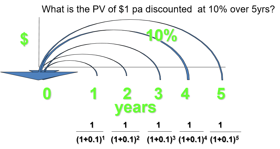
This cash flow can be present valued by the following formula:
| Years | PV $1 @ 10.00% |
|---|---|
| 5 | 3.79 |
| 10 | 6.105 |
| 50 | 9.92 |
| 75 | 9.992 |
| 100 | 9.999 |
The Capitalisation Method
- Income producing properties assessed based on the present value current and future income.
- Capitalisation rates are deduced from market evidence.
- Capitalisation method assumes
- income consistent in perpetuity
- risk profile of income remains constant
Determinants of cap rates
-
opportunity cost of capital
-
risk perceptions and preferences among investors considering space and capital market
-
growth expectations
- rental cash flows
-
good cash flow growths? Sustainable income?
- reversion price (capital gains)
6) Mortgage Factor
- What is the repayment of $200,000 loan to be spread in equal instalments annually in arrears over 5 years assuming an interest of 8% per annum (interest compounded annually)?
Instalment =
Instalment = $50091.29
- How much you have to pay in an amortising loan to repay principle over a period of time
- What is the ratio of the total amount of money you pay to the principle? In this example,
DISCOUNTED CASH FLOWS
Discounted Cash Flow (DCF) analysis
- Discounted cash flow (DCF) analysis applied to commercial property
The Direct Capitalisation method which has been covered in detail is the traditional tool for the Valuation of investment properties. You should all by now be totally conversant with the formula
- This method relies on current and historical data. However, investors typically look to the future to assess potential returns and the associated risks.
Traditional evaluation tool for investment properties
Implicit v Explicit Risk Assumptions
-
The Discounted Cash Flow (DCF) Method is an alternative approach to the valuation of investment class properties. In many respects it is essentially the same as Direct Capitalisation, but a major difference is that all assumptions made in the DCF model are explicit and readily capable of being altered.
-
Therefore the DCF method lends itself to “sensitivity analyses”, under which key variables are changed to assess the impact on the outcome. In this way, the results can be said to be more or less sensitive to specific key variables. This is also known as a “what if” analysis.
- Cap method is primary
- DCF in income producing properties Main difference
- all assumptions in bundled discount rate into an implict figure
- can perform a sensitivity analysis in a DCF, change key assumptions
Which cashflows?
-
DCF looks at current and future cash flows (positive and negative) and brings then back to a present value. This requires projections of future incomes and costs which are influenced by many factors.
-
Economic performance (national, regional & local)
-
Interest Rates
-
Business/economic/property cycles
-
Supply and Demand
- Projection of future income
- Projection of future costs
- Assumptions on supply and demand
- macroeconomic performance Lost of factors which will influence projections and income for cash flows
-
Both Direct Capitalisation and DCF are focused on accurately establishing a net income figure and converting that to a capital sum.
-
Where Direct Capitalisation uses a market derived Cap Rate with implicit growth and risk assumptions, DCF employs a discount rate which incorporates the investor’s required rate of return with all cash flow assumptions being explicit.
DCF Model
-
But first, we need to spend some time to build our DCF model. The major elements of the DCF model are:
-
Cash Flows (positive and negative)
-
Escalation Factors
-
The Holding Period
-
A Terminal Value, and
-
The Discount Rate
-
Measuring Financial Performance
- Escalation factors - how much does your income and expenses escalate?
- Lease mechanism the same for simplicity - indexed to the same percentage
- consumer price index, evaluation at market
- negative cash flows and costs
- referential to market? Need to figure out market Holding period
- model cash flows for a period of time
- Best way of doing this to adopt a period which is generic for that type of period
- adopt a 10 year holding period if other people hold for 10 years, e.g.
- DCF & holding period - if something major has happened before the holding or after the holding, it can skew your modelling
- might want to reconsider duration of holding period
- massive losses on capital improvements in last years, might want to increase investment horizon
- overall, referable to the sector, or major capital improvements Terminal Value
Cashflows
- Cash flows are based on current amounts which are then escalated at specific rates over the study period (holding period) of the investment.
- They can be positive or negative depending on the type of cash flow. Income from all sources is positive and can include rent, outgoings recovery, parking fees, naming/signage rights, electricity profit, proceeds of sale, etc.
- Negative cash flows, opex, vacancy allowances, Incentives (depending on type), agency letting fees, purchase and selling costs, etc.
- The timing of these cash flows is critical to the result of the analysis. Matters to be considered include the “rest periods” (eg., yearly, quarterly, monthly rests, etc) and
Rest period
- yearly, quarterly, monthly
- a commercial property with 40 tenants and all paid monthly & 10 year investment horizon
- 4800 separate incomes over the life of the spreadsheet
- can simplify and look at this yearly
- can look monthly, quarterly yearly
- Quarterly or yearly is completely acceptable
-
Whether the cash flows fall at the beginning, end or middle of the period. We must also remember at this stage that the current period is by convention Period “0”.
-
Let us start with a very simple cash flow model. Assume we are evaluating an office building with a gross rent of $100pa and outgoings of $30pa.
| Items | 0 |
|---|---|
| Gross Rental Income | 100 |
| Outgoings | 30 |
| Net Income | 70 |
Escalation Factors
-
Escalation factors are the specific rates at which the various cash flows will be projected over the study period. Different cash flows will grow at differing rates over time.
-
Forecasting of rental rates is particularly difficult and relies heavily on the skill and expertise of the analyst.
In above case, no escalation factor Assume you got the $70 at the end of the year, but had to pay $30 upfront
- Rental rates are heavily influenced by the demand and supply characteristics of their own specific market sector.
- Property cycles are generally different for the various property sectors (ie. commercial office, industrial, retail, residential, tourism, etc) and also for different regions for specific sectors (ie. commercial office in Brisbane, Sydney, Melbourne, etc and Brisbane CBD, Fringe, Qld regional, etc).
- Costs such as maintenance and other outgoings items tend to follow general inflationary trends and therefore the CPI index is a suitable escalator for such cash flows.
We can now return to our simple cash flow model, starting with projections of rental growth and CPI over a study period of 5 years.
| Period | 1 | 2 | 3 | 4 | 5 | 6 | 7 |
|---|---|---|---|---|---|---|---|
| Rental Growth | 2.0% | 5.0% | 7.0% | 2.0% | 0.0% | 0.0% | |
| CPI | 0 | \2.5% | 2.7% | 3.0% | 2.4% | 2.2% | 0.0% |
positive cash flow different ot negative cash flows (rental growth vs CPI)
Apply escalation rate to our cash flows:
| Period | 1 | 2 | 3 | 4 | 5 | 6 | 7 |
|---|---|---|---|---|---|---|---|
| Gross Rent | 100 | 102 | 107.10 | 114.60 | 116.89 | 116.9 | |
| Outgoings | 30 | 30.75 | 31.58 | 32.53 | 33.31 | 34.04 | |
| Net Income | 70 | 72.15 | 75.52 | 72.08 | 83.58 | 82.86 |
Holding Period
-
Unlike Direct Capitalisation which employs a Cap Rate to capitalise a net income figure in perpetuity, DCF utilises a specific holding period tailored to the time that the investor intends to keep the investment before selling it, or disposing of it in another manner (eg. redevelopment).
-
This holding period is also known as the Investment Horizon
DCF uses a specific holding period, works out the cash flows over that period (holding period) known as the investment horizon
Terminal Value
- We will shortly see that the asset is hypothetically “sold” at the end of the holding period. This will also explain why we have added an additional year (year being the first period, then year 6 in the model must be outside the holding period).
Basic static capitalisation
- In order to “close off” the cash flow series, the model requires that a terminal value is added in the final period. This terminal value represents a hypothetical sale at the end of the investment holding period.
- This is a proxy for the value that the asset still has at the end of the study period, and without including this asset value, the DCF will be incomplete.
- Note that Direct Capitalisation assumes the asset is held in perpetuity and therefore does not need to include a terminal value.
- We use the Direct Capitalisation method to establish the terminal value.
Where CV is the terminal value.
capitalisation to determine net terminal value Make assumptions - building will be more obselete, allow higher vacancy, figure out what the market value is in the future have to pick a yield - have to decide and make assuptions based to the property, market in future, etc.
Terminal Value
- Adding a terminal value to our model. Assume a current cap rate of say, 8.5% and therefore a softer terminal yield of say, 9.5% for our model.
Year 6 net income is:
- Gross Rental = $116.89
- Outgoings = $34.04
- Net Income = $82.85
Therefore
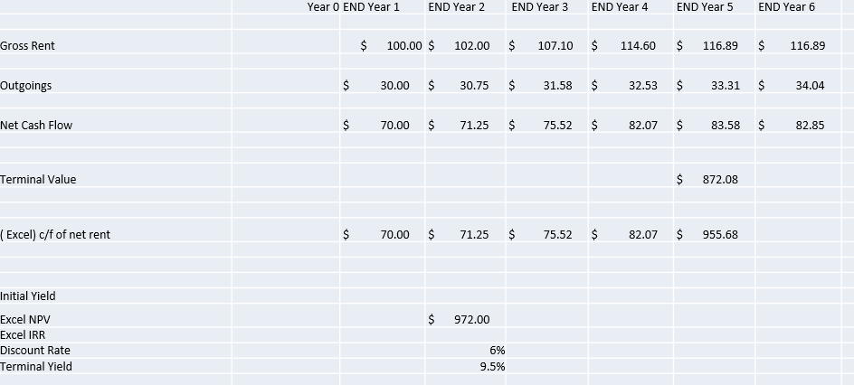
Cashflows including terminal value
- Our model now looks like this this, and only lacks a discount rate to complete it.
| Period | 1 | 2 | 3 | 4 | 5 | 6 | 7 |
|---|---|---|---|---|---|---|---|
| Gross Rent | 100 | 102 | 107.10 | 114.60 | 116.89 | 116.9 | |
| Outgoings | 30 | 30.75 | 31.58 | 32.53 | 33.31 | 34.04 | |
| Net Income | 70 | 72.15 | 75.52 | 72.08 | 955.68 | 82.86 |
- adding terminal value to the property
Discount rate
- We now move on to the final and possibly most critical of the elements of DCF, the discount rate.
- The discount rate is employed to bring a future amount, or a future series of cash flows to a present value.
- Therefore, the cash flows in our simple model can also be “discounted” back to a present value.
But how do we establish the discount rate?
Each one of the years of income, need to discount it back
- PV of future amount, apply to each year incomes
-
“When valuing property the discount rate may be regarded as comprising two portions, namely, a risk -free rate component reflecting the minimum level of return required as compared to minimal risk investment such as Government long term bonds, and a risk premium reflecting the additional level of return required to offset the inherent risks of property investment… There are several ways in which the discount rate may be calculated, including:
-
Risk-free Rate + Risk Premium
-
Weighted Average Cost of Capital
-
Client’s Input
-
Analysis of Sales Evidence.”
API Practice Standard – “Discounted Cash Flows”
- Risk free plus risk premium component
- WACC
- Have a client tell you the preferred discount rate
From the preceding definitions, we can glean the following:
-
The discount rate as applied in the property industry is the return required by the investor (the probable purchaser of the property). It incorporates opportunity cost (the return that the investor could have received on an alternative investment) inflation and risk. In selecting a discount rate, due consideration should be given to property market forces, particularly:
- Property characteristics of the subject property
- Tenants Covenant
- Prevailing and likely future property market conditions
- General economic conditions.
Return the investor requires for that property
We can also say that the main methods of structuring the discount rate are:
Risk-free rate (10 year Commonwealth Bond rate used as a proxy) plus a risk premium Opportunity Cost plus inflation plus risk Analysis of comparable sales evidence (not easy) Survey of market sentiment WACC (Weighted Average Cost of Capital) – used by the finance industry Client specific.
Easiest way
- risk free + risk premium
- If you can find WACC, use that as well
- Enough industry reports that outline a range of discount rates
- For our purposes, it is easy to establish discount rates referable to The Risk-free rate (10 year bonds) plus a risk premium.
- The risk premium will be dependent on property specific risk factors such as the age and quality of the property and Tenant’s Covenant.
Look at the challeges associated with maintaining the income stream uncertain and challenging - risk is much higher
Financial Performance
Financial Performance-Net Present Value (NPV)
-
We should be aware by now of discounting and the term Present Value. We must now introduce a variation on the PV concept, the Net Present Value (NPV).
-
The NPV is the sum of all cash flows in a DCF model discounted by the required rate of return. It is the difference between the present value of all positive and negative cash flows or capital sums included in a DCF model.
-
The NPV can be a positive or negative outcome itself, but generally, in a feasibility study, when an NPV is positive, the investment proposal is acceptable and when negative it is not (or it may be marginal)
Model and all of the income and expedntiures will be,
- work out the financial performance, sum of all cash flows of the DCF model
NPV calculation
A – Using the Financial Calculator Discount each individual cash flow from the series using:
- FV = 70 (first cash flow, the second etc)
- I = 6
- N = 1, 2, 3, 4, 5
- PV = ?
Follow this through for all the cash flows, increasing the “n” by 1 each time. You should end up with:
- 70.00 = 66.03
- 71.25 = 63.41
- 75.25 = 63.41
- 82.07 = 65.01
- 955.68 = 714.14
- Total (NPV) = 971.77
Using the model before with the 5 years of various cash flows,
Timing of Cashflows
-
Timing of Cash Flows (Beginning or End of Period):
-
You will have noted that in the previous NPV calculations, we have discounted the year 1 cash flow. This is legitimate provided that the cash flows have been received (or assumed) at the end of the period.
-
With annual “rests”, and monthly rental payments, it is a moot point as to whether cash flows should be deemed to be at the beginning or end of the period.
-
When using the NPV formula in Excel, be aware if the first period is to be discounted. For this reason, the NPV‘s calculated in the simple model have been based on the end of period “rests”.
When looking at rest periods and p.a. interest rate
Cap rate vs Discount rate
-
The Cap Rate vs the Discount Rate
-
By now we should be starting to see that the cap rate and discount rate are two completely separate concepts, and must NEVER be interchanged.
-
Even though the cap rate is a type of discount rate it is a simple multiplier derived from comparable market sales,
-
However the DCF the discount rate is the investor’s target rate of return for a specific investment vehicle. The discount rate may also be derived from market evidence by the valuer when performing a valuation using DCF, but in this case it is reversing the DCF process to ascertain the discount rate employed.
Two separate concepts
- cap rate 'all risks rate'
- DCF is discounting a cash flow of a particular investment vehicle
Applications for DCF model
-
For Valuations: The NPV is the valuation figure. Acquisition costs must be deducted.
-
For Feasibility Studies:
A project can be assessed using DCF by determining whether all the projected costs and benefits discounted at the target rate of return(hurdle rate) result in a positive NPV. -
Internal Rate of Return (IRR): The IRR is the discount rate at that point where the present values of all positive and negative cash flows result in a zero NPV. The IRR needs both a positive and negative cash flow to function and must include all acquisition costs as well as net disposal proceeds.
Are you getting a sufficient return to justify the investment?
- PV of all positive and negative cashflows that result in a 0 or positive NPV
Sensitivity Analyses
-
DCF analyses readily lends itself to the “what if” process, where key variables/assumptions can be changed to see if the outcome (NPV or IRR) has been radically altered.
-
Different variables will have different impacts under the assumptions made, and by undertaking a sensitivity analysis, the risks inherent in the project can be quantified to some degree.
-
One important aspect (and criticism of DCF) is that, due to the discounting process, cash flows later in the time series have a much lesser impact on the NPV or IRR. Terminal values come into this category.
What if? scenarios
- delay refurbishment, improvements etc.
- change inputs and assumptions