Lecture 10 - Topic 8 - Behavioral Explanations for Anomalies
[Behavioral Explanations for Anomalies]
- Brief Introduction: Behavioral Explanations for Anomalies
- Earnings Announcements and Value vs. Growth
- What is behind lagged reactions to earnings announcements
- What is behind the value advantage
- What is Behind Momentum and Reversal
- Daniel-Hirshleifer-Subrahanyam Model
- Grinblatt-Han Model and Explaining Momentum
- Barberis-Shleifer-Vishny Model and Explaining Momentum and Reversal
- Rational Explanations
- Important Risk Adjustment
- Fama-French Three Factor Models/Factor Zoo – Tutorial
Traditional Finance vs behavioural finance
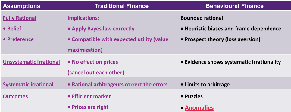
- Should be able to access them correctly
- Should be unsystematic
- Even if they form a consensus, arbitrageurs should be able to correct the price
- Prices should always be efficient
Behavioural finance
- Behavioural factors effecting our decisions
EMH: Empirical Challenges
Anomalies
- Excess volatility: Shiller (1981) and Le Roy (1981)
- Stock prices are far more volatile than would be justified by simple model in which prices are equal to the discounted expected future dividends.
- Equity premium puzzle
- Time series stock market predictability puzzle
- Cross-sectional price-scaled anomalies: value premium
- Over- and under-reaction [Today’s focus]
- Seasonal effects
- “Twin shares” with different prices
- Challenges to EMH
- Always comparing to EMH
- First three, talk about next week
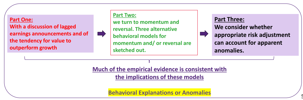
Introduction: Behavioral Explanations or Anomalies
- Four key anomalies reviewed were:
- the small-firm effect;
- lagged reactions to earnings announcements;
- value versus growth;
- momentum and reversal
Review of Trading Rules that Have Shown to be Effective.
- Small cap portfolios vs. large cap portfolios?
- Small cap wins out!
- Portfolios formed based on P/Es:
- Low P/Es do better!
- Earnings announcements momentum:
- Reaction to extreme announcements is slow!
- Value vs. growth portfolios
- (usually, value firm has a high book-to-market, and a growth firm has a low book-to-market):
- Go for value!
- Predictable serial correlation:
- Medium-term momentum!
- Long-term winners vs. losers:
- Reversals: losers become winners!
- Small firms tend to outperform the big ones
- Big firms should have more information and outperform in general
- Investor tend to underreact to earnings announcements
- Don't react immediately, have momentum
What is Behind Value Advantage?
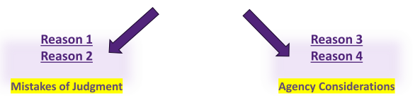
- It has been suggested that there are four main reasons why retail and institutional investors have favoured glamour stocks over value stocks:
- They are committing judgment errors in extrapolating past growth rates too far into the future and are thus surprised when value stocks shine and glamour stocks disappoint. This is so-called “expectational error hypothesis”
- Because of representativeness, investors may assume that good companies are good investments These first two reasons are mistakes of judgment. Likely individual investors are more subject to committing them than institutional investors.
- P/E ratio
- have a high PE ratio, paying a lot more compared to their book value
- indicates high growth rate - considered a 'growth' stock
- Low P/E ratio considered an undervalued stock
- Simply looking at the price, look really cheap - new firm, may no be great, etc.
- Literature looks at two streams
- Looking at the past performance - firm is still going to have a growth rate in the future
- Assume a constant/terminal growth rate in DCF, e.g., will have higher prices for the stock
- Thinking that because of high growth rate, higher growth in the future and give it a higher price and you are surprised when it underperforms in the future
- Representativeness
- For an investment to be good, generate high returns - but should be reflected in the share price
- If the price is really high now - high growth rate currently
What is Behind Value Advantage?
Next two reasons (Reason 3 and Reason 4) are due to agency considerations (rational reasons to shy away from value):
- Because sponsors view companies with steady earnings and buoyant growth as prudent investments, so as to appear to be following their fiduciary obligation to act prudently, institutional investors may shy away from hard-to-defend, out-of-favour value stocks.
- Also because of career concerns, institutional investors, who are evaluated over short horizons, may be nervous about tilting too far in any direction thus incurring tracking error. A value strategy would require such a tilt and may take some time to pay off, so it is in this sense risky.
- Should work in the best interest for their client
- Not easy - have performance pressure, have to show they are generating income
- find another agent/manager
- Prefer to invest in growth stocks, easier to justify
- Managers don't have a lng time horizon
- Evaluate the performance at least once a year
- different to long term investment
- To show they are good at what they are doing, easy to realise their returns
- Value stocks, not quick for the price to be corrected
- Safer/less risky to invest in growth stocks compared to value stocks
Explaining Long-Run Value Outperformance
- Take a growth stock with a high P/E or P/B.
Such stocks have a period of anticipated higher-than-normal growth.
- What if market overestimates length of supernormal growth period?
When it becomes clear that mean reversion is occurring, growth stocks deteriorate. Similar story (in reverse) can be told for value stocks.
- In long run, value stocks outperform growth stocks
- If investors are too optimistic, push the value even higher
- Price should always come back to fundamental value
- Short term period of time, reach too far then the price of stocks will crash
Introduction: Behavioral Explanations or Anomalies
- Recall the existence of intermediate-term momentum and long-term reversal.
- Putting these results together suggests that investors first underreact and then overreact.
- In essence we have a combination of the underreaction seen in the earnings announcement literature and the overreaction requiring reversal that we see in the value literature.
- In the market, don't always see momentum and reversal
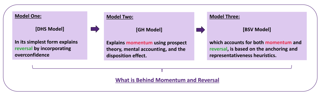
Daniel-Hirshleifer-Subrahmanyam (DHS) Model: Explaining Reversal
DHS model is based on overconfident investors overestimating the precision of their own private signals.
== > This leads to a negative serial correlation in price movements (i.e., reversal).
DHS model details
- Begin in equilibrium at t=0.
- At t=1 private noisy information appears (one can assume informed investors undertake some analysis generating private signals).
Formally, the private information at t=1 is:
- where θ is a mean-zero random variable with variance 𝝈𝜽𝟐 that represents the change in the true value of the security
- At t=2 true value of security is revealed.
- Signal is a combination of true information and noise
- Idea of why we have reversal, we over estimate our private signal
- Overconfident, information you have is more accurate than it is
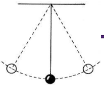
Black dot, equilibrium price
- like a pendulum, push back to the opposite direction
true value theta plus some error epsilon
- normally distributed
- Signal is observed imperfectly because of a mean-zero noise term with variance .
- Overconfidence is a factor because informed traders exaggerate in their own minds the accuracy of their private signal,
Using instead of where, <
- Given the risk neutrality of the informed traders, the price at t = 1 settles at the expected value of θ conditional on .
- At t = 2, the price reaches the true value of the security
- difference is between overconfident investors
- miscollaborated - narrow range of precision
- Overestimate the accuracy - give a really precise answer
- Calculate the variance - going to give a much narrower variance and you think the variance is going to be narrower
- Variance is another measure of risk level
- Variance for level of overconfidence investors is
- If overconfident, <
DHS Model: Price Response at t = 1
Consider the price at t = 1. The challenge is to separate the information from the noise.
- Intuitively, if is low relative to , it will be rational to believe that the signal is primarily the true change in value.
- On the other hand, if ε is high relative to , it will be rational to believe that the signal is primarily noise. In the former case, it will be rational to alter valuations almost as much as s 1 .
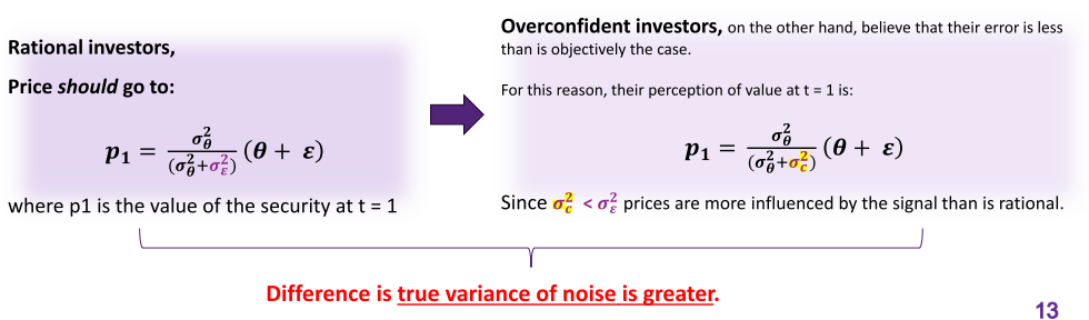
- Overconfident investors will assign a lower variance than the rational one
- If variance is smaller, signal will be greater
Example
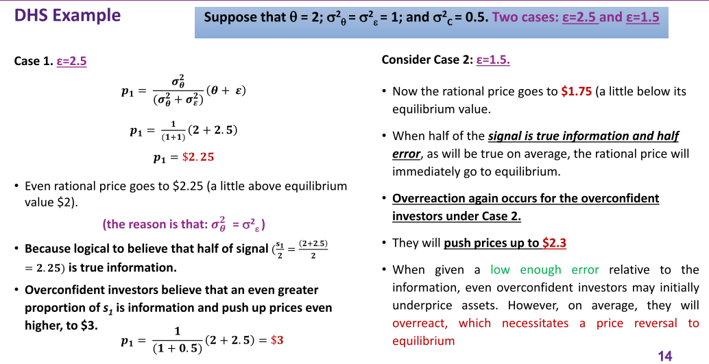
- Compare what overconfident and rational investors will think
- Calculate for a rational investor, what we will expect the price to be
- Most cases, would expect investors to overreact to news
- What is the difference between true investors and noise
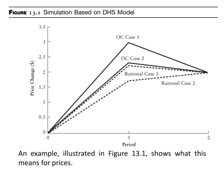
Price Path Graphs
The DHS model offers a number of testable implications.
Solid lines in the graph show price paths assuming that overconfident traders drive prices.
Broken lines show price paths assuming no overconfidence.
- For example, managers should issue shares when they believe their stocks to be overvalued and buy them back when they believe them to be undervalued.
- Should they issue new shares?
- When it crashes, pay less to investors
Grinblatt-Han Model (to explain momentum)
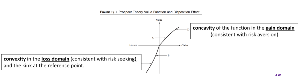
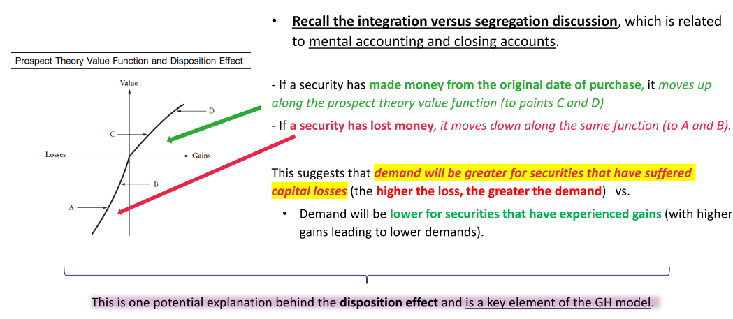
Grinblatt-Han model (hereafter GH), is based on prospect theory, mental accounting, and the disposition effect.
- In brief, the tendency for winners (losers) to be sold too quickly (slowly) suggests a delayed reaction to good/bad news, because reference-point-influenced investors have demand curves that reflect recent performance.
- Because of how we treat past winners and losers
- Past winning and losing performance is going to affect us
- Going to be more risk averse
- If a stock is not performing well, going to hold for longer
- Momentum in having the price continuing to decrease
- underreaction causing us to have momentum
Grinblatt-Han Model – Intrinsic Value
- Consider the (intrinsic) value () of a security in the GH model. It follows a random walk, only changing as relevant news () arrives:
- Demand comes from two groups of investors: rational investors (R) and those who are influenced by Prospect Theory and Mental Accounting (PT/MA). The first group has the following demand function:
-
where is the demand coming from rational investors at t; and pt is the share price at t. Note that b > 0 reflects the slope of the rational demand curve. To the extent that value exceeds price, rational investors will demand more units.
-
PT/MA investors account for the second component of overall market demand:
- D(PT/MA)t is demand at t arising from those investors who are influenced by prospect theory and mental accounting. Here, ref t is the reference point and λ (>0) denotes the relative importance of the capital gain component to PT/MA investors. Note that, if ref t > p t , demand is higher since the price is in the risk-seeking domain.
- intrinsic value is larger than the price, then it is undervalued
- larger the difference between the intrinsic value and the price, the more we will want it
- mental accounting + disposition effect
Investors are affected by their reference point and the stock market price
- if the second term is negative, going to cause the demand to decrease
- Even if something is losing, causing you to buy more of it
Market Price
- If PT/MA investors; are μ% of all investors; we aggregate demand over the two groups; normalize supply at one unit; and clear the market; the resulting equilibrium price is:
To interpret, the market price is a weighted average of value and the reference point.
- Underreaction to news is clear. Say, beginning from a steady state (where f t = p t = ref t ), positive news pushes up value.
- Price will react in the same direction, but it will be held back somewhat by the reference point (which, as will be shown, moves more slowly).
- Only over time will price reach the right level. Because this takes time, we have momentum.
- Further, the more PT/MA investors there are (higher μ), and the more important is the capital gain component to them (higher λ), the more influential is the reference point and the greater is the underreaction.
- Intrinsic value should reflect true price
- Previously it was 1
- Price should immediately reflect
- Rationally should adjust our reference point, which we don't always do
- old number into equation - number is underreacting
Grinblatt-Han Model – Intrinsic Value
- This enters the model in the following reference point adjustment equation, where the speed of adjustment is v:
- For example, assume that a particular PT/MA investor bought shares at $5 (so her reference point is $5).
- The price now rises to $7 for a capital gain of $2, but her reference point remains at $5.
- Suppose she needs cash and sells her shares to another PT/MA investor for $7.
- His reference point will be $7, which is his purchase price (not hers).
- Therefore, over time because of trading, the reference point moves toward the market price.
- How quickly they adjust their reference point to market value
- v - speed of adjustment
Grinblatt-Han Model – Simulation Based on GH Model
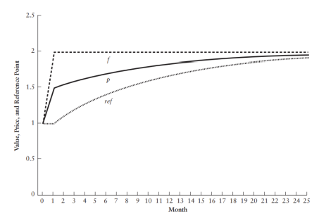
Figure 13.3 shows the evolution of prices and reference points over the next 24 months (to t = 25).
- Price moves toward value, but it does so gradually because PT/MA investors fixate on the reference point, which moves more slowly.
- The reader will of course realize that real-world securities never exhibit momentum as “clean” as in this example. The reason is that new additional information (affecting ft) is often arriving.
- Start to adjust reference point, slowly reach intrinsic value
Grinblatt-Han Model – Intrinsic Value

Nevertheless, a stock’s unrealized capital gain is likely to be highly correlated with past returns, so standard momentum is easily implied by the model. Capital gain should be a better predictor of future returns than past returns.
- Indeed, Grinblatt and Han find this to be true: the momentum effect disappears once the PT/MA disposition effect is controlled for.
- Still, one weakness of the GH model is that it only explains momentum, not reversal.
For this reason, we turn to the final model, which explains both momentum and reversal. BSV model: Explaining momentum/reversal
- Talking about momentum model only
Barberis-Shleifer-Vishy (BSV) Model: Explaining Momentum/Reversal
Recall sun and clouds example:
- At first people were too anchored.
- Then they were too influenced by new evidence. What about earnings?
- Anchoring and conservative adjustment dictates that investors are slow to change views on earnings.
- First surprise tends to be followed by a few more.
- Eventually recency and base rate underweighting take over and past performance is extrapolated into the future.
- Overreaction: The current high-growth/low-growth period is viewed as longer than is logical. Their Model leads to a world where investors at first underreact, and then overreact to salient news.
Markets overreact slowly!!!
- Still anchored on initial information
- then overreact to new information that causes reversal
BSV Model Formalises This Story
- Earnings follow a random walk:
- Changes in earnings are +y or –y with equal probability
- But investors, being coarsely calibrated, believe that stocks switch between two regimes.
Suppose we assume that a random walk holds for earnings (nt):
- Regime 1. Earnings mean-revert:
Given a positive (negative) earnings change, there is a low probability of another positive (negative) earnings change in the next period. Underreaction.
- Regime 2. Earnings are persistent:
Given a positive/negative earnings change, there is a high probability of another positive/negative earnings change in the next period. Overreaction
- adjusting probability of probability, changes regime
At all points in time, individuals must guess whether the world is in Regime 1 or 2. Estimated probabilities will rise and fall as events unfold:
- Alternating changes (e.g., +y, –y, +y, –y) will lead people to believe that Regime 1 is in effect.
- While a sequence of like earnings changes (e.g., +y, +y, +y, +y; or -y, –y, -y, –y) will lead people to believe that Regime 2 is in effect.
- Start to predict in regime
- Another series of events for series of positive or negative, will always be in regime 2
- It can be shown that if earnings changes are the same at both t and t + 1, the perceived probability that regime 1 is in place is the following function of the parameters of the model:
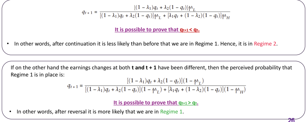
- transition probability into regime 1 next period
- Likelihood of being in regime 1
- If you believe the chance of us being in regime 1 next period is less than the chance of us being in regime 1 now, means that we think we will be in regime two
- If you think the chance that we will be in regime one is higher next period compared to what we have now, then we will continue to be in Region one.
- Turning to valuation, it is assumed that all earnings are returned to investors in the form of dividends. Using a standard dividend discount model, value is:
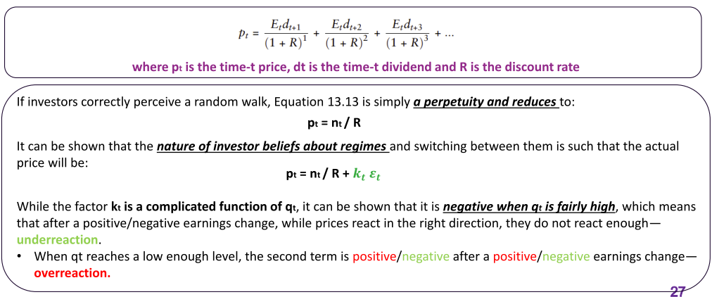
- assume 100% of earning distributed out as dividends
- Rationally speaking
- Second part in green pushing the price away from fundamental
Simulation Based on BSV Model
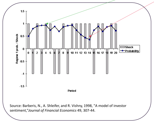
To see how the model works in terms of the revision over time of the probability that the world is in regime 1, refer to Figure 13.4.
Note that q t rises after a sign switch but falls after a sign continuation.
- line is the
- When the earning kept on swapping, when we start to see some consistent performance, probability starts to decrease, more chance of being in regime 2
- How this beliefs affects overreaction and underreaction
Explaining Momentum and Reversal
Investor beliefs about regime will dictate prices:
- When investors think Regime 1, they underreact to earnings changes
- When investors think Regime 2, they overreact to earnings changes
So, this model can explain both underreaction and overreaction.
And momentum and reversal empirical regularities can be simulated.
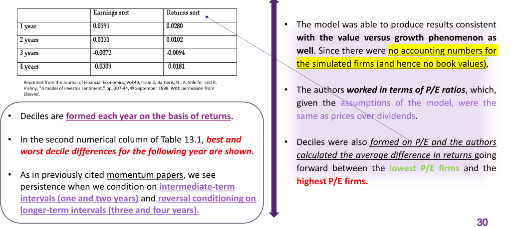
- Consistent with momentum papers, Barberis, Shleifer, and Vishny find intermediate-term (1 & 2 years) momentum, and reversal for longer-term intervals (3 & 4 years)
- General theory is the same
- Overeaction will cause reversal
- Underreactions, not moving quick enough
- Don't need to know too much
Simulated Returns from Earnings and Returns Sorts Based on BSV Model
Rational Explanation - Inappropriate Risk Adjustment
- Early tests only assume that appropriate risk adjustment only considers market or beta risk (as in CAPM).
- Joint-Hypothesis Problem Illustrated with a Casino Example:
- Slot machines at a casino advertise a -2% return, but a true loss is -5%.
- Over time, gamblers adjust their expectations to this 5% loss, making it the new norm.
- An economist testing for efficiency might mistakenly use the advertised -2% as the benchmark, leading to incorrect conclusions about market efficiency.
- On top of beta,
Inappropriate Risk Adjustment.
- Fama and French's 1992 Paper:
Challenged the then-accepted CAPM model, suggesting it didn't work anymore. CAPM indicates only a security's beta should impact expected returns. Their data (from 1963-1990) contradicted this, showing no positive relation between stock returns and market betas.
- Multi-dimensional Stock Risks:
Findings suggest that stock risks have multiple dimensions, including size and the book-to-market equity ratio. This led to the development of the Fama-French three-factor model.
- Anomalies' Interpretation:
Anomalies in stock returns either indicate investor errors or improper risk adjustment.
Fama-French Three Factor Model
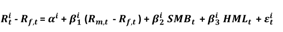
-
Where the return on security or portfolio at is :
-
The risk-free rate at t is
- Market Return:
- Value vs. growth
- Small cap vs. large cap
-
One issue is what underlies the second and third Fama-French risk factors. Fama and French suggest that different aspects of so called “distress risk” are being captured.
-
But, these distressed stocks do not perform appreciably worse in bad times.
- adjust for cap size and value of the premium
- Should also capture distress risk
- Should also measure overall risk
- Smaller firms would be more constrained
- size should capture everything
Conclusion
- Post-announcement earnings drift appears to be driven by anchoring on the part of investors and analysts.
- The value premium is likely due to both behavioral and agency-related institutional factors.
- A number of theoretical models have been formulated to account for momentum and reversal.
- The DHS model explains reversal using overconfidence; the GH model explains momentum using prospect theory, mental accounting, and the disposition effect; and the BSV model accounts for both momentum and reversal and is based on the anchoring and representativeness heuristics.
- Much of the empirical evidence is consistent with the implications of these models.
- Another view is that risk has been improperly accounted for in the research that has identified these anomalies, and a proper treatment of risk will render these anomalies as merely risk premiums.
- The Fama-French three-factor model has value and small cap as risk factors over and above market risk.
- Under Fama-French, value is a risk factor, not an anomaly. Some have questioned whether greater exposure to the value factor really does entail additional risk.
- Momentum is not credibly accounted for by any risk-adjustment technique.
- IMPORTANT
- Don't worry too much about understanding the model